Writing Parquet That VertiPaq Likes

This rabbit hole started with a simple observation: VertiPaq seemed to like parquet produced by delta-rs more than parquet produced by DuckDB — and that drove me nuts. delta-rs was at the time a niche library for nerds; Fabric didn’t even have a Python notebook. The mental model was simple: write with Spark, get V-Order, get the best possible layout for Power BI.

It is 2026; Fabric is more widespread, and there are simply more patterns and use cases:

  • New Fabric workspaces default Spark to the writeHeavy resource profile, which does not write V-Order.
  • Customers — especially on smaller SKUs — routinely write with delta-rs from Python notebooks.
  • Reading tables written by Snowflake, Databricks and BigQuery through Direct Lake is a production pattern.

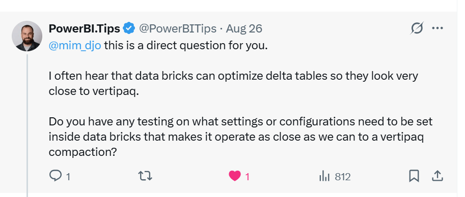
So “what parquet is friendly to Vertipaq” is now a legitimate data engineering question — I can’t tell you how happy I was when I read this tweet 🙂
The short version

  1. Row groups of a few million rows : 2–6M rows per group; never go above 16M, VertiPaq’s segment ceiling.
  2. Dictionary-encode every column — and make the file footer say so.
  3. One global ORDER BY, lowest-cardinality columns first, date up front. No clustering, no Z-ordering, none of that.
  4. Delta vs Iceberg does not matter. Only the parquet inside the table matters.

Method

I treated VertiPaq as a black box and did what experimental science does with a phenomenon it doesn’t understand: change one variable, measure, repeat. Nothing here is confidential or internal — every number was measured from the outside, on tables anyone can rebuild.

One more thing changed this year: AI became genuinely useful for this kind of work, because it never gets bored. Sweeping writers × row-group sizes × file sizes × sort orders across hundreds of runs is exactly the tedium it doesn’t feel.

Two experiments.

  • First: figure out why VertiPaq preferred delta-rs output.
  • Second: run multiple writers and vary row-group count, file size and ordering, measuring cold, warm and hot query cost.

Caveat. Hot behaviour is well documented — after all, it is the same in-memory format as import mode — so I am more interested in cold runs (first touch of a fresh model), even though most real-world traffic is hot: a live model transcodes once and then serves from RAM.

The datasets are rather smallish — the biggest table here is around 600M rows. As a data analyst I have always dealt with small data, so I am optimising for the workload I actually care about.

How Direct Lake reads your parquet

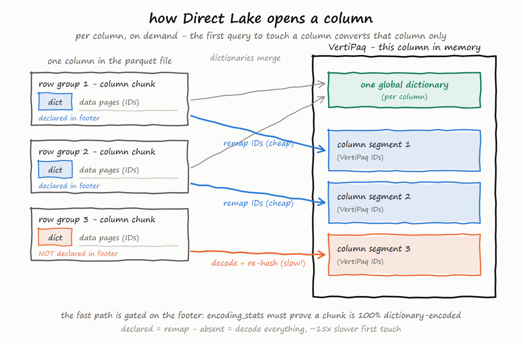
The mechanism that explains almost every finding. Transcoding is per column, on demand: the first DAX query to touch a column that is not yet in memory converts that column only into VertiPaq’s in-memory format. The column’s per-row-group parquet dictionaries are merged into one global VertiPaq dictionary, and each row group of the column is loaded as one resident column segment, remapping parquet data IDs onto VertiPaq IDs on the way in. Every query after that scans the segments the transcode produced. Query latency — and capacity consumption — is therefore a property of how the parquet was written.
Findings

Dictionary encoding is the big one

VertiPaq is itself a dictionary-based engine. When a chunk arrives dictionary-encoded, the transcode merges the parquet dictionary into the column’s global one and remaps the data IDs — it never decodes the values. Anything else has to be decoded and re-hashed, value by value, at load time. On a single 144M-row DECIMAL(18,4) column, PLAIN measured 618.6 MB against 423.1 MB dictionary-encoded — ~200 MB extra and a re-encode, on one column.

The surprise is that the encoding alone isn’t enough: the declaration is part of the encoding. The engine takes the cheap remap path only when the footer’s encoding_stats prove a chunk is entirely dictionary-encoded without decoding its pages. DuckDB’s writer emitted no encoding_stats at all until duckdb#24957 (merged 2026-08-24, currently in main only). That PR measures the cold first-touch of a 142M-row dictionary string column falling from 10,857.5 ms to 689.3 ms — about 15×, with identical pages. The attribution was verified the hard way: synthesising only that footer field into an otherwise unmodified file reproduces the speedup. A second PR, duckdb#24645 (merged 2026-08-10), adds a data_page_size_limit option — before it, DuckDB often wrote one huge data page per column chunk.

Row-group size: a tension between cold and hot

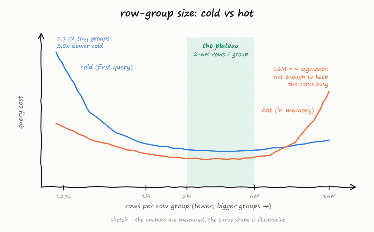
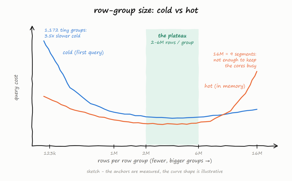
There is no single best size, but both ends fail measurably. Every row group is one more dictionary merge and one more segment to set up per column, which is why tiny groups murder the cold tier: the same DuckDB in the same notebook was 3.5× slower cold (96,503 ms vs 27,785 ms) when a library default sliced a 144M-row table into 1,172 groups of ~123k rows. At the other end, 16M rows — VertiPaq’s segment ceiling — was the worst sorted geometry measured: nine segments starve the scan pool. Cold prefers slightly bigger groups than hot, but very big groups are bad for both.

Power BI doesn’t disclose how many cores it uses, so the practical rule is: enough row groups to keep the cores busy. On the 144M-row table, warm query time stepped down between 19 and 24 groups (≈5,700 ms → 3,221 ms), and 72 groups bought nothing over 24. Hence the plateau: 2–6M rows per group.
A global sort keeps paying after the data is in memory

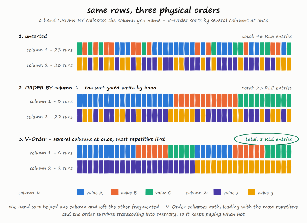
Transcoding does not change row order — it is essentially a working data copy into memory. So a sort applied at write time survives into the resident segments, which is why ordering matters for hot runs too, not just for compression.

A single global ORDER BY with low-cardinality columns first (and a preference for date) produces long RLE runs. It is not V-Order — but in some cases it is good enough. When V-Order does engage, what it’s worth depends on the surface — column count × categorical skew — not row count: on a skewed 17-column taxi table it collapsed the most repetitive column to 3,371× fewer runs; on a near-unique 5-column table it left row order untouched and still shrank files 16%. One caution from the sweep: an alternative sort key cut file size a further 30% and bought statistically zero query time — sort for the columns your queries filter on, not for size on disk.

This is also the cleanest way to see what V-Order’s reorder actually is. A hand-written ORDER BY collapses the column you name and leaves the others fragmented; V-Order sorts by several columns at once, most repetitive first — the taxi measurement above is its signature, runs falling off exactly as an encoding-driven sort predicts.
VertiPaq doesn’t like ragged row groups

delta-rs closes a file the moment the size cap is hit, truncating the in-progress row group — measured writing groups at 0.43× their declared rows. A truncated group isn’t just small; it makes segment sizes uneven, exactly the non-uniform scan load you were sizing row groups to avoid. I’ve proposed a fix in delta-rs#4677 — still open, and opt-in — which rolls files only on row-group boundaries.

Dynamic row group size at write time are very hard.

I built a personal package, duckrun, using delta-rs and DuckDB and tried a clever optimisation. The plan: before writing a query’s result, estimate its row count and compute the perfect row-group size on a 1M–16M scale. It failed completely, because query planners are bad at estimating output size — DuckDB estimated ~14.9M rows for a table that actually held 143,980,961, 9.7× too low — so the “optimised” geometry was off by an order of magnitude. Derive geometry from an exact count (the table you’re rewriting, the Delta log) — never from an estimate. Not only that: in an initial version the cost of the estimation was nearly the same as writing the table 🙂

Anyway, I endup writing 6M as the default row group everywhere, i feel it is a good enough compromise

Takeaway

V-Order is usually understood as row reordering — and the reordering is real; the hard part is not the reordering itself but doing it fast (that’s the secret sauce basically), to be super clear, V-order is a local sort, not global

But it is not only that: a V-Order write also sets the row-group geometry and runs the encoding pass, keeping a declared dictionary on every column.

Two consequences follow:

 If you write with a Fabric engine, turning V-Order on is a no-brainer, and honestly, it should be the default in my personal opinion.

measured here at ~8% of build compute for up to 2.8× less query capacity (1,332 vs 3,769 CU on identical data) — the write premium is paid once, while queries pay every day. I do wish it were simpler to turn on: changing the Spark write profile is not obvious, and a lot of users don’t even know it is there. As someone who used VertiPaq for more than a decade with zero knowledge of columnar data structures, I suspect there must be a better way.

If you write with anything else — Snowflake, Databricks, delta-rs, DuckDB — my hope is that there will be more public specifications on how to optimize parquet layout for VertiPaq.

Thanks to Krystian Sakowski for answering my silly questions 🙂

Links

First Look at OneLake Diagnostics

While preparing for a presentation about the FabCon announcement, one item was about OneLake Diagnostics. all ll I knew was that it had something to do with security and logs. As a Power BI user, that’s not exactly the kind of topic that gets me excited, but I needed to know at least the basic, so I can answer questions if someone ask 🙂

Luckily, we have a tradition at work , whenever something security-related comes up, we just ping Amnjeet 🙂

He showed me how it works , and I have to say, I loved it. It’s refreshingly simple.

You can download the notebook here:


You just select a folder in your Lakehouse and turn it on.

That’s it , the system automatically starts generating JSON files, neatly organized using Hive-style partitions, By default, user identity and IP tracking are turned off unless an admin explicitly enables them. You can find more details about the schema and setup here.


What the Logs Look Like

Currently, the logs are aggregated at the hourly level, but the folder structure also includes a partition for minutes (even though they’re all grouped at 00 right now).

Parsing the JSON Logs

Once the logs were available, I wanted to do some quick analysis , not necessarily about security, just exploring what’s inside.

There are probably half a dozen ways to do this in Fabric ; Shortcut Transform, RTI, Dataflow Gen2, DWH, Spark, and probably some AI tools too, Honestly, that’s a good problem to have.

But since I like Python notebooks and the data is relatively small, I went with DuckDB (as usual), but Instead of using plain DuckDB and delta_rs to store the results, I used my little helper library, duckrun, to make things simpler ( Self Promotion alert).

Then I asked Copilot to generate a bit of code for registering existing functions to look up the workspace name and lakehouse name from their GUIDs in DuckDB, using SQL to call python is cool 🙂


The data is stored incrementally, using the file path as a key , so you end up with something like this:

import duckrun

con = duckrun.connect('bigdata/tpch.lakehouse/dbo')

onelake_logs_path = (
    'abfss://bigdata@onelake.dfs.fabric.microsoft.com/'
    'tpch.Lakehouse/Files/DiagnosticLogs/OneLake/Workspaces/*/'
    'y=*/m=*/d=*/h=*/m=*/*.json'
)

Then I added only the new logs with this SQL script:

try:
    con.sql(f"""  
        CREATE VIEW IF NOT EXISTS logs(file) AS SELECT 'dummy';
        SET VARIABLE list_of_files =
        (
            WITH new_files AS (
                SELECT file
                FROM glob('{onelake_logs_path}')
                WHERE file NOT IN (SELECT DISTINCT file FROM logs)
                ORDER BY file
            )
            SELECT list(file) FROM new_files
        );
        SELECT * EXCLUDE(data), data.*, filename AS file  
        FROM read_json_auto(
            GETVARIABLE('list_of_files'),
            hive_partitioning = true,
            union_by_name = 1,
            FILENAME = 1
        )
    """).write.mode("append").option("mergeSchema", "true").saveAsTable('logs')
except Exception as e:
    print(f"An error occurred: {e}")

1- Using glob() to collect file names means you don’t open any files unnecessarily , a small but nice performance win.

2- DuckDB expand the struct using this expression data.*

3- union_by_name = 1 in case the json has different schemas

4- option(“mergeSchema”, “true”) for schema evolution in Delta table


Exploring the Data

Once the logs are in a Delta table, you can query them like any denormalize table.

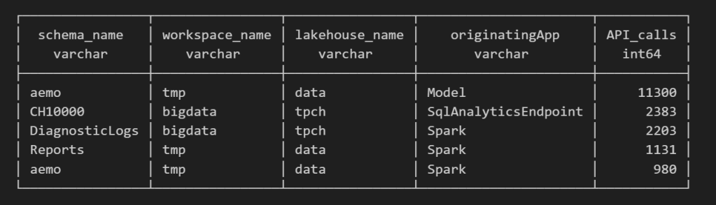
For example, here’s a simple query showing API calls per engine:

Note : using AI to get working regex is maybe the best thing ever 🙂

SELECT
    regexp_extract(resource, '([^&/]+)/([^&/]+)/(Tables|Files)(?:/([^&/]+))?(?:/([^&/]+))?', 4) AS schema_name,
    get_workspace_name(workspaceid) AS workspace_name,
    get_lakehouse_name(workspaceid, itemId) AS lakehouse_name,
    originatingApp,
    COUNT(*) AS API_calls
FROM logs
GROUP BY ALL
ORDER BY API_calls DESC
LIMIT 5;

Fun fact: OneLake tags Python notebook as Spark.
Also, I didn’t realize Lineage calls OneLake too!

as I have already register Python functions as UDFs, which is how I pulled in the workspace and lakehouse names in the query above.


Takeaway

This was just a bit of tinkering, but I’m really impressed with how easy OneLake Diagnostics is to set up and use.

I still remember the horrors of trying to connect Dataflow Gen1 to Azure Storage ,that was genuinely painful (and I never even got access from IT anyway).

It’s great to see how Microsoft Fabric is simplifying these scenarios. Not everything can always be easy, but making the first steps easy really gives the feature a very good impression.

First Look at Geometry Types in Parquet

Getting different parties in the software industry to agree on a common standard is rare. Most of the time, a dominant player sets the rules. Occasionally, however, collaboration happens organically and multiple teams align on a shared approach. Geometry types in Parquet are a good example of that.

In short: there is now a defined way to store GIS data in Parquet. Both Delta Lake and Apache Iceberg have adopted the standard ( at least the spec). The challenge is that actual implementation across engines and libraries is uneven.

  • Iceberg: no geometry support yet in Java nor Python, see spec
  • Delta:  it’s unclear if it’s supported in the  open source implementation (I need to try sedona and report back), nothing in the spec though ?
  • DuckDB: recently added support ( you need nightly build or wait for 1.4)
  • PyArrow: has included support for a few months, just use the latest release
  • Arrow rust : no support, it means, no delta python support 😦

The important point is that agreeing on a specification does not guarantee broad implementation. and even if there is a standard spec, that does not means the initial implementation will be open source, it is hard to believe we still have this situation in 2025 !!!

Let’s run it in Python Notebook

To test things out, I built a Python notebook that downloads public geospatial data, merges it with population data, writes it to Parquet, and renders a map using GeoPandas, male sure to install the latest version of duckdb, pyarrow and geopandas

!pip install -q duckdb  --pre --upgrade
!pip install -q pyarrow --upgrade
!pip install geopandas  --upgrade
import sys
sys.exit(0)

At first glance, that may not seem groundbreaking. After all, the same visualization could be done with GeoJSON. The real advantage comes from how geometry types in Parquet store bounding box coordinates. With this metadata, spatial filters can be applied directly during reads, avoiding the need to scan entire datasets.

That capability is what makes the feature truly valuable: efficient filtering and querying at scale, note that currently duckdb does not support pushing those filters, probably you need to wait to early 2026 ( it is hard to believe 2025 is nearly gone)

👉Workaround if your favorite Engine don’t support it .

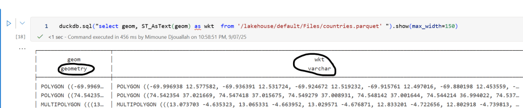
 A practical workaround is to read the Parquet file with DuckDB (or any library that supports geometry types) and export the geometry column back as WKT text. This allows Fabric to handle the data, albeit without the benefits of native geometry support, For example PowerBI can read WKT just fine

duckdb.sql("select geom, ST_AsText(geom) as wkt  from '/lakehouse/default/Files/countries.parquet' ")

For PowerBI support to wkt, I have written some blogs before, some people may argue that you need a specialized tool for Spatial, Personally I think BI tools are the natural place to display maps data 🙂

Does a Single-Node Python Notebook Scale?

I was giving a presentation about Microsoft Fabric Python notebooks and someone asked if they scale. The short answer is yes. You can download the notebook and try it for yourself. For the long answer, keep reading.

The dataset I used contains the last seven years of Australian electricity market data. Although it’s public, the government agency only keeps archives for two months. I had saved the data during a previous job and kept it around as a hobby. It’s a great real-world workload with realistic data distribution. The CSV files are messy. Technically, they’re more like reports, with different sections stacked on top of each other and varying numbers of columns. That’s often what you encounter in real projects, not the neat, well-structured datasets you see in demos.

For example, being able to read a CSV file with a variable number of columns is a critical feature. Yet this rarely gets mentioned in synthetic benchmarks.

To create a clean environment for testing, I copied the data from one Lakehouse in onelake to a brand-new workspace. I could have used a shortcut, but I wanted to start from scratch. The binary copy took just 2 minutes, with no transformations, which gives a throughput of 1.4 GB per second. That’s pretty good for a 150 GB uncompressed dataset.

The default configuration for Fabric Python notebooks includes 2 cores and 16 GB of RAM. That’s roughly the same size as Google Colab. But you can easily increase the number of cores to 4, 8, 16, 32, or even 64. At 64 cores, you get nearly half a terabyte of RAM. That’s a serious machine.

The job itself is simple. Ingest and process the data using several Python engines, then save the result as a Delta table. The raw data has around one billion records, and you end up extracting 311 million. If your engine cannot push down filters to the CSV level, you’re going to have a hard time. The trick here is not to be fast, but to avoid doing unnecessary work.

I used the following engines: DuckDB, Daft, Polars, CHDB (basically ClickHouse for Python), DataFusion, PyArrow, and Pandas. Technically, Pandas is not ideal here because you can’t pass a list of files without using a loop. But I had used it for nearly seven years, so I kept it for sentimental reasons.

I’m fairly confident using all of these engines except PyArrow and DataFusion. Their syntax is very intimidating, and I probably missed some configuration settings. I couldn’t get them to use more than a single thread, so CPU utilization stayed very low.

Results

  • Polars support streaming writes, but doesn’t allow exporting a record batch. This means the Delta writer has to load all data into memory. It works fine with 32 cores and 256 GB of RAM, but you’ll run into out-of-memory issues with 16 cores and below.
  • Chdb 3.5 added a user friendly way to export arrow record batch, it is the first release so still some bugs, for example got an error with 2 cores, I am sure it will get fixed soon
  • Daft is the only engine that supports native writing to Delta. It uses the Deltalake package only to commit the transaction log. The actual Parquet write is handled by the engine itself.
  • DuckDB preserves the sort order of the input files. it is trick to appeal to Pandas users who care about index ordering. For best performance though, you should turn this off. (Honestly, I think it should be off by default)
  • DuckDB exports Arrow tables by default. You need to explicitly use record_batch(). I’ve lost count of how many out-of-memory issues I’ve solved just by changing the export format.
  • Overall, DuckDB delivered the best performance, especially considering it’s not even writing Parquet files directly. It simply streams Arrow data to the writer.

When I first ran the test with DuckDB and saw it finish in under 4 minutes, I thought I made a mistake. It wasn’t until CHDB finished in under 5 minutes that I realized these engines are seriously impressive.

We’re talking about 625 MB per second for processing and ingestion on a single node.

Another key observation: using DuckDB and Daft, even with just 16 GB of RAM, the data was processed correctly. It took about an hour, but it worked without errors, that’s 10 X the size of the RAM

To verify correctness, I simply checked the total sum of a column and the number of records. Everything checked out.

Choosing the Right Size

Now that I know these notebooks work, choosing the right size becomes more nuanced. Surprisingly, the cheapest configuration in term of capacity usage was the 2 cores 🙂

In practice though, using more compute makes sense. A single node has no concept of fault tolerance. If something goes wrong, you need to restart the entire job. Personally, I’m not a fan of long-running jobs. Too many things can go wrong. I used 2 cores just to make a point. That said, using 64 cores doesn’t make much sense either. You’re doubling your compute cost to save 30 seconds.

One more thing: while Daft scales down very well, it doesn’t seem to scale up as efficiently as I had hoped. Ideally, you want a flat performance curve. The total amount of work is fixed, so adding more cores should just reduce execution time. I know the reality is more complex. It’s not easy to keep all processors busy at higher scales.

What This Means

As you may have guessed, I’m a big fan of single-node setups and DuckDB. But I don’t want just one engine to dominate every benchmark or deliver results that no other engine in its class can match. That’s why I was genuinely excited by Daft’s performance. I’m also looking forward to seeing Polars and CHDB add Arrow streaming support.

To be honest, I look at the world from a storage perspective. More competition between engines is a good thing. All of these tools are open source under the MIT license. Most of them can write to Delta in one form or another. and as a user you can choose any engine you want, I think that’s a fantastic thing to have.

So yes, Python notebooks do scale. The experience is far from being perfect, and there’s still room for improvement. But scalability is not something you should worry about, unless of course you are really doing real big data, then you go distributed 🙂 DWH and Spark are robust options in Fabric.

Edit : tested with chdb 3.5 which has support for arrow streaming