Iceberg on a single node is coming together

For a long time, whenever I tried to use Iceberg outside the JVM ecosystem, something I needed seemed to be waiting for the next release. It took longer than I hoped, but lately I have been able to get much further with the engines I use.

chDB can authenticate to OneLake with a token, Polars now runs all 22 queries in this benchmark, and DuckDB’s cache feels like absolute magic on the second pass. I still ran into bugs, but I could run both reads and writes across several engines against the same Iceberg catalog.

I took two of my notebooks and port them to GitHub Actions as python script across DuckDB, Polars, chDB, LakeSail, Spark and Daft. One runs analytical queries; the other reads CSVs and writes Iceberg tables. I wanted to see how each handled the workloads on a small 4-core runner.

The data lives in OneLake. Reading through its Iceberg REST catalog is already available; the write support I used is still in private preview.

Both benchmarks run on a public 4 vCPU / 16 GB runner. The engines connect to the catalog either directly or through pyiceberg. OIDC federation provides a token per job, so there is no client secret to store. The same approach should work with other Iceberg REST catalogs, provided the engine supports their storage and authentication.

The code, the raw JSON of every run and the charts are in djouallah/lakehouse_benchmark.

Reading: TPC-H-like queries at SF10

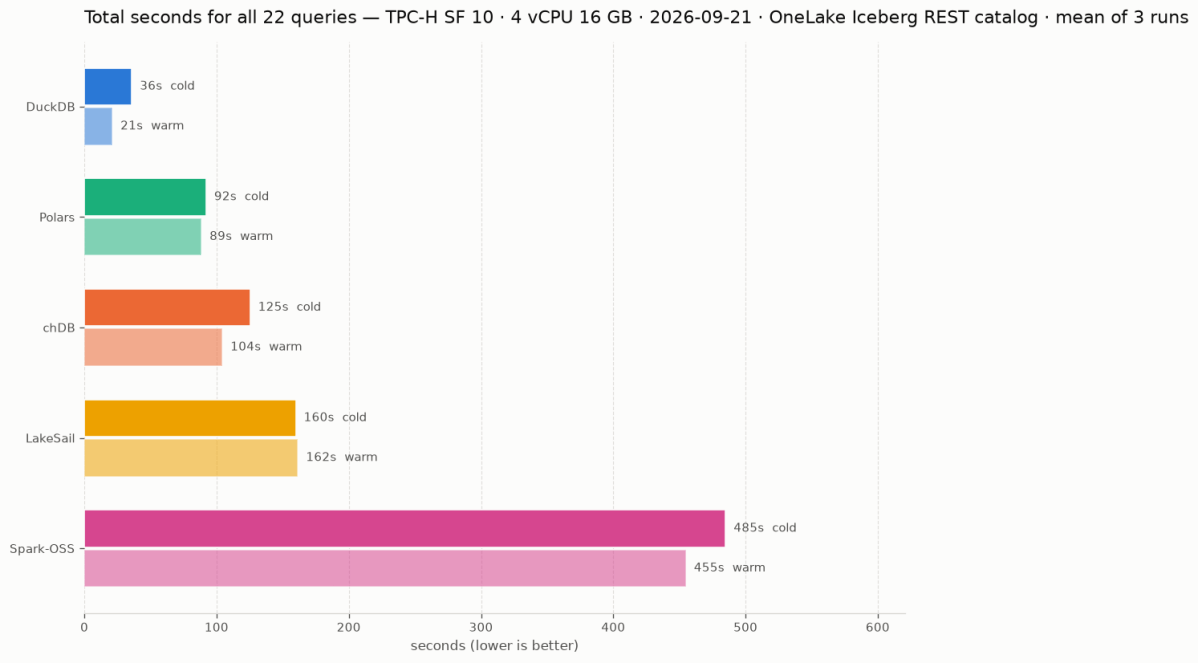
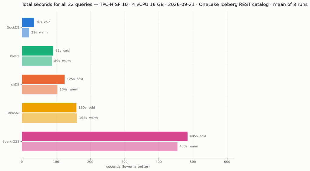
The tables are generated with tpchgen, uploaded as Parquet and registered with pyiceberg’s add_files. DuckDB and LakeSail could have written them just fine, but I wanted to stay neutral. Each engine attaches the catalog, runs the 22 queries, then runs the same 22 again immediately. Those are the cold and warm passes below; catalog attach time is excluded. The chart and the table are the mean of three runs on 20 and 21 September 2026. This is a small single-node comparison, not an official TPC-H benchmark.
EngineVersionColdWarm
DuckDB2.0.0 dev35.9s21.3s
Polars2.0.0-rc.292.1s88.6s
chDB4.4.0125.4s104.5s
LakeSail0.7.1159.9s161.6s
Spark-OSS4.1.3484.9s454.9s

Spark open source, not to be confused with Fabric Spark, is a single-node JVM on 4 cores here. Thanks to AI, running Spark locally is no longer a scary experience. Unfortunately Daft is missing: at 0.7.25 it runs 16 of the 22 queries, because l_extendedprice * (1 - l_discount) overflows its decimal precision ceiling of 38 (Daft#7532). I like Daft and would love to include it in the full query comparison once this is fixed. It does complete the ETL workload below.

Writing: Light ETL

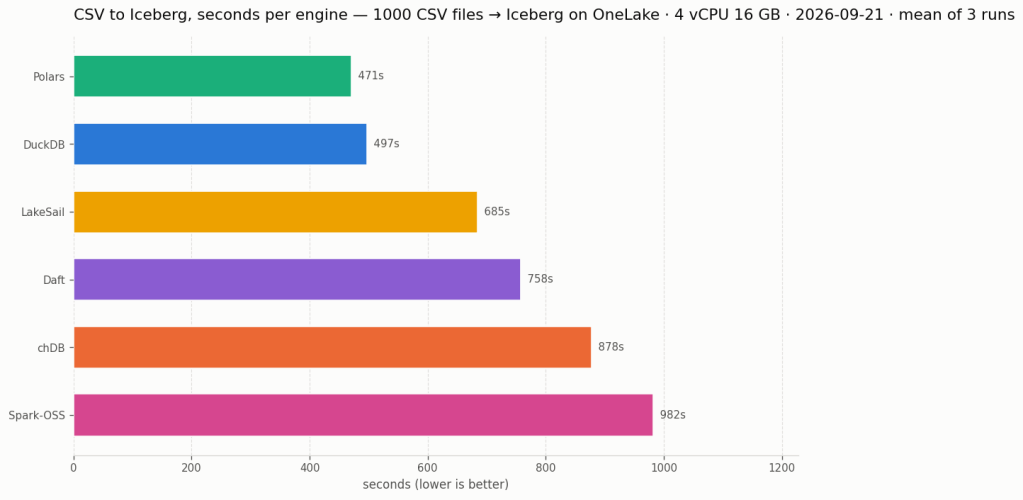
1000 daily AEMO CSV files, 52 GB, are landed once in the lakehouse Files/ section. Each engine reads all of them, filters, casts and writes one Iceberg table of 149,146,763 rows through the same catalog. DuckDB, LakeSail and Spark have their own Iceberg writer. chDB and Polars stream Arrow batches into pyiceberg. Daft has its own writer over a pyiceberg table.
EngineLoad
Polars470.8s
DuckDB497.4s
LakeSail684.5s
Daft757.9s
chDB878.1s
Spark-OSS982.2s

Every engine ends with the same row count. Load time includes recreating the table, reading the CSVs, transforming, writing and committing; session setup and catalog attach are timed separately. There is one load pass per engine, and the chart and the table are the mean of three runs. Snapshot isolation and concurrent writes will have to wait for another blog. The Iceberg write path used here is in private preview.

Random learnings, in no particular order

  • DuckDB needed AZURE_TRANSPORT_OPTION_TYPE=curl on this Linux runner. Without it the Iceberg attach succeeds and every data-file read fails with a message that looks exactly like a missing credential. Setting the transport fixed it. I had not seen this in the Fabric notebook.
  • chDB returned 41 rows for Q13, everybody else 42. ClickHouse defaults join_use_nulls=0 and fills unmatched outer-join cells with default values instead of NULL. The row-count smoke test caught this, and the benchmark now sets join_use_nulls=1.
  • The catalog cache settings do not all mean the same thing. I configured a 15-minute lifetime, but LakeSail’s “table cache” caches the table listing, not the loaded table. It still loads table metadata on every statement, adding REST requests even on the warm pass (sail#2629).
  • Daft’s six query failures come from decimal arithmetic. CTEs, EXISTS and correlated subqueries all work. It also rejects backticks outright, which looked like a total dialect failure until I read the error. Separately, its Azure URI parser drops the container on OneLake hosts; the bench works around it with az:// paths. The proposed fix is Daft#7533.
  • Nothing is partitioned, on purpose. The pyiceberg streaming append used here only supports unpartitioned tables. A first version that materialised batches to partition by year took the 16 GB runner down at 100 files. So every engine writes the same unpartitioned shape and year stays a plain column.

Spark, and why it has no native accelerator here

Spark-OSS is 4.1.3 with Iceberg 1.11 and hadoop-azure 3.4.2. I also looked at Comet and Gluten/Velox, but could not use either for this benchmark.

  • Comet supports Spark 4.1 and ships a native Iceberg reader, but its readable schemes are file, s3, s3a, gs, oss. An abfss table is declined at planning time and runs on the JVM as if the plugin were not there. I left Comet out because it could not accelerate these scans. Filed as datafusion-comet#6058.
  • Gluten/Velox has a Velox ABFS connector, but I could not find a published package for Spark 4.x to test (This basically what Fabric NEE uses)

Conclusion

All six engines completed the CSV-to-Iceberg load. Five completed all 22 read queries; Daft completed 16. Being able to try this many engines against one catalog, with the data staying in OneLake, is what I find exciting. chDB’s token support and Polars running all 22 SQL queries give me more options for the notebooks I already use.

DuckDB was fastest on the reads, and on the load it traded first place with Polars from run to run. DuckDB’s read total fell from 36s to 21s on the second pass, about 40%. The other engines improved less, and LakeSail’s warm pass came out slightly slower than its cold one. That makes repeated reads worth testing separately from a one-pass load. It does not tell us exactly what each engine cached or how many bytes it fetched; chDB also has a filesystem cache configured here.

For my ETL workload, the cache does not matter: read the new files, transform them and write the table.

If you want to see how much things have changed, have a look at these TPC-H SF10 results from four years ago.

Note: The write benchmark requires access to the private preview used here coming soon.

Does a Single-Node Python Notebook Scale?

I was giving a presentation about Microsoft Fabric Python notebooks and someone asked if they scale. The short answer is yes. You can download the notebook and try it for yourself. For the long answer, keep reading.

The dataset I used contains the last seven years of Australian electricity market data. Although it’s public, the government agency only keeps archives for two months. I had saved the data during a previous job and kept it around as a hobby. It’s a great real-world workload with realistic data distribution. The CSV files are messy. Technically, they’re more like reports, with different sections stacked on top of each other and varying numbers of columns. That’s often what you encounter in real projects, not the neat, well-structured datasets you see in demos.

For example, being able to read a CSV file with a variable number of columns is a critical feature. Yet this rarely gets mentioned in synthetic benchmarks.

To create a clean environment for testing, I copied the data from one Lakehouse in onelake to a brand-new workspace. I could have used a shortcut, but I wanted to start from scratch. The binary copy took just 2 minutes, with no transformations, which gives a throughput of 1.4 GB per second. That’s pretty good for a 150 GB uncompressed dataset.

The default configuration for Fabric Python notebooks includes 2 cores and 16 GB of RAM. That’s roughly the same size as Google Colab. But you can easily increase the number of cores to 4, 8, 16, 32, or even 64. At 64 cores, you get nearly half a terabyte of RAM. That’s a serious machine.

The job itself is simple. Ingest and process the data using several Python engines, then save the result as a Delta table. The raw data has around one billion records, and you end up extracting 311 million. If your engine cannot push down filters to the CSV level, you’re going to have a hard time. The trick here is not to be fast, but to avoid doing unnecessary work.

I used the following engines: DuckDB, Daft, Polars, CHDB (basically ClickHouse for Python), DataFusion, PyArrow, and Pandas. Technically, Pandas is not ideal here because you can’t pass a list of files without using a loop. But I had used it for nearly seven years, so I kept it for sentimental reasons.

I’m fairly confident using all of these engines except PyArrow and DataFusion. Their syntax is very intimidating, and I probably missed some configuration settings. I couldn’t get them to use more than a single thread, so CPU utilization stayed very low.

Results

  • Polars support streaming writes, but doesn’t allow exporting a record batch. This means the Delta writer has to load all data into memory. It works fine with 32 cores and 256 GB of RAM, but you’ll run into out-of-memory issues with 16 cores and below.
  • Chdb 3.5 added a user friendly way to export arrow record batch, it is the first release so still some bugs, for example got an error with 2 cores, I am sure it will get fixed soon
  • Daft is the only engine that supports native writing to Delta. It uses the Deltalake package only to commit the transaction log. The actual Parquet write is handled by the engine itself.
  • DuckDB preserves the sort order of the input files. it is trick to appeal to Pandas users who care about index ordering. For best performance though, you should turn this off. (Honestly, I think it should be off by default)
  • DuckDB exports Arrow tables by default. You need to explicitly use record_batch(). I’ve lost count of how many out-of-memory issues I’ve solved just by changing the export format.
  • Overall, DuckDB delivered the best performance, especially considering it’s not even writing Parquet files directly. It simply streams Arrow data to the writer.

When I first ran the test with DuckDB and saw it finish in under 4 minutes, I thought I made a mistake. It wasn’t until CHDB finished in under 5 minutes that I realized these engines are seriously impressive.

We’re talking about 625 MB per second for processing and ingestion on a single node.

Another key observation: using DuckDB and Daft, even with just 16 GB of RAM, the data was processed correctly. It took about an hour, but it worked without errors, that’s 10 X the size of the RAM

To verify correctness, I simply checked the total sum of a column and the number of records. Everything checked out.

Choosing the Right Size

Now that I know these notebooks work, choosing the right size becomes more nuanced. Surprisingly, the cheapest configuration in term of capacity usage was the 2 cores 🙂

In practice though, using more compute makes sense. A single node has no concept of fault tolerance. If something goes wrong, you need to restart the entire job. Personally, I’m not a fan of long-running jobs. Too many things can go wrong. I used 2 cores just to make a point. That said, using 64 cores doesn’t make much sense either. You’re doubling your compute cost to save 30 seconds.

One more thing: while Daft scales down very well, it doesn’t seem to scale up as efficiently as I had hoped. Ideally, you want a flat performance curve. The total amount of work is fixed, so adding more cores should just reduce execution time. I know the reality is more complex. It’s not easy to keep all processors busy at higher scales.

What This Means

As you may have guessed, I’m a big fan of single-node setups and DuckDB. But I don’t want just one engine to dominate every benchmark or deliver results that no other engine in its class can match. That’s why I was genuinely excited by Daft’s performance. I’m also looking forward to seeing Polars and CHDB add Arrow streaming support.

To be honest, I look at the world from a storage perspective. More competition between engines is a good thing. All of these tools are open source under the MIT license. Most of them can write to Delta in one form or another. and as a user you can choose any engine you want, I think that’s a fantastic thing to have.

So yes, Python notebooks do scale. The experience is far from being perfect, and there’s still room for improvement. But scalability is not something you should worry about, unless of course you are really doing real big data, then you go distributed 🙂 DWH and Spark are robust options in Fabric.

Edit : tested with chdb 3.5 which has support for arrow streaming

An Excel User’s Perspective on Lakehouse Architecture

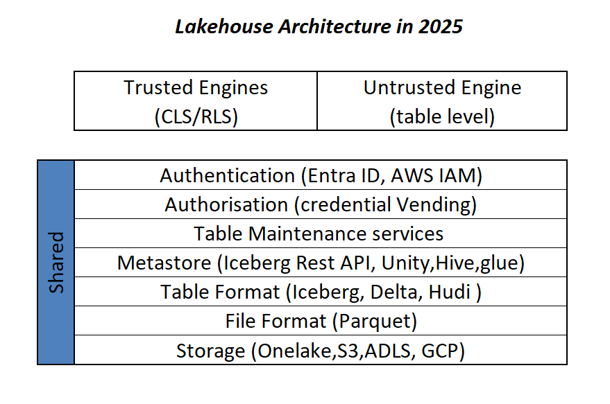
This is more or less the industry consensus on how a Lakehouse architecture should look in 2025.

By now, it’s become clear that Parquet is the de facto standard for storing data, and using an object store to separate storage from compute makes a lot of sense.

Another interesting development is how vendors want to package this offering. Storage vendors saw an opportunity to do more—after all, there’s no law that says the metastore belongs to the data warehouse! So you get things like S3 Table and Cloudflare R2, which I think is a good thing, especially if you’re a smaller analytics vendor. Life becomes much easier when table maintenance is done upstream, allowing you to focus solely on making the query engine faster.

Encouraging things are also happening in the table format space. I know a bit about Iceberg and Delta, but not much about the others. One very interesting development is Iceberg adopting deletion vectors from Delta in the V3 spec, while Delta will requires a catalog for read and write (at least for catalog managed table). I like to call it the “Icebergification” of Delta.

Another trend is the Delta Java writer making it easier to auto-generate Iceberg metadata. and Xtable is doing the same regardless of the delta writer, At this stage, one could argue: why do we need two table formats that are becoming virtually identical?

Data Analyst—How About Me?

These improvements mostly impact the write path, which is primarily managed by data engineers. But what about data analysts and end users?

if you have Fabric OneLake, you can use Direct Lake in OneLake mode. Marco has a great article about it. It’s a fantastic improvement compared to the initial version of Direct Lake. However, it doesn’t solve the problem if your data is hosted in an S3 table or BigQuery Iceberg table. Yes, you can create a shortcut to OneLake and read it from there, but that still depends on a data engineer setting it up.

Now imagine a world where an Excel, Tableau, or Power BI Desktop user (or any arbitrary client tool) can just point to a Lakehouse using a standard API, discover tables, read data, and build reports. Honestly, this isn’t a big ask , we already have this when connecting to databases using ODBC, and I don’t see any technical reason why we can’t have the same experience with Lakehouses.

We Already Have This API

For me, the most promising development in the Lakehouse ecosystem is the Iceberg Catalog REST API, and I genuinely hope it becomes a standard—just like ODBC is today (and hopefully ADBC in the future, but that’s another topic).

Again, speaking as a data analyst, I want my tools to support the read part of the API—just the ability to list tables and scan a table. That’s all. I have zero interest in how the data is stored or which table format is used. The catalog should be smart enough to generate metadata on the fly.

The Good News

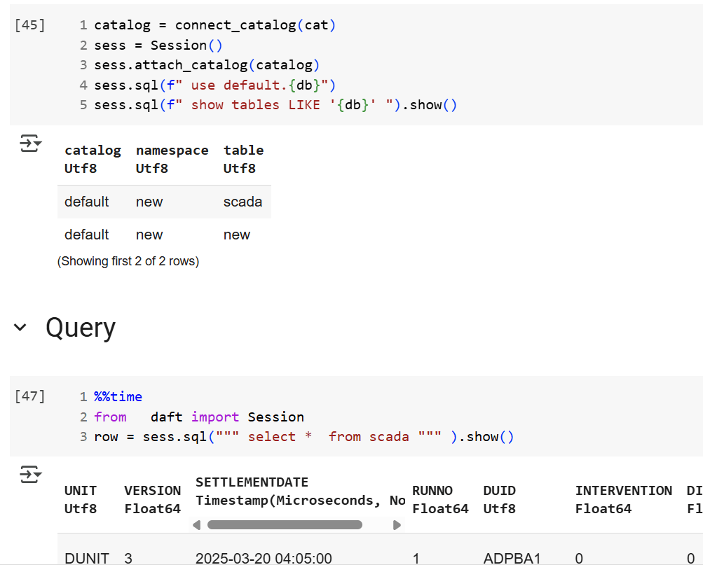
We’re getting there—at least if you’re using a Python notebook. Here’s an example where I use the same Iceberg REST API to query a table from four different Lakehouse implementations using Daft.

def connect_catalog(cat):
  match cat:
    case 'polaris':
      catalog = load_catalog(
              'default',
              uri= polaris_endpoint,
              warehouse='dwh',
              scope = 'PRINCIPAL_ROLE:data_engineer' ,
              credential= polaris_key
            )
    case 's3':
      catalog = load_catalog(
              'default',
              **{
                "type": "rest",
                "warehouse": s3_warehouse ,
                "uri": "https://s3tables.us-east-2.amazonaws.com/iceberg",
                "rest.sigv4-enabled": "true",
                "rest.signing-name": "s3tables",
                "rest.signing-region": "us-east-2"
              }
            )
    case 'uc':
      catalog = load_catalog(
               'default',
              token = token ,
              uri = endpoint,
              warehouse = 'ne'
              )
    case 'r2':
      catalog = RestCatalog(
              name = 'default',
              token = token_r2 ,
              uri = endpoint_r2,
              warehouse = r2_warehouse
              )
  return catalog

Then, I run a standard SQL query using Daft SQL.

Final Thoughts

It took Parquet a decade to become a standard. We may or may not have a single standard table format—and maybe we don’t need one. But if we want this Lakehouse vision to become mainstream, then everyone should support the Iceberg Catalog REST API, at least for read operations.

Create Iceberg Table in Azure Storage using PostgreSQL as a catalog

Just sharing a notebook on how to load an iceberg table to ADLSGen2, I built it just for testing iceberg to delta conversion.

Unlike Delta, Iceberg requires a catalog in order to write data, there are a lot of options, from sqlite to full managed service like Snowflake Polaris, unfortunately pyiceberg has a bug when checking if a table exists in Polaris, the issue was fixed but it is not released yet.

SQLite is just local db, and I wanted to read and write those tables using my laptop and Fabric notebook, fortunately PostgreSQL is supported

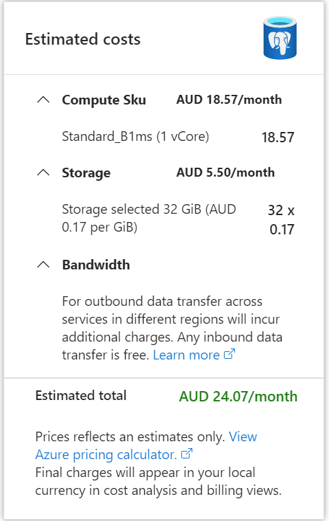
I spinned up a PostgreSQL DB in Azure, I used the cheapest option possible, notice here, iceberg catalog doesn’t store any data, just a pointer to the latest snapshot, the DB is used for consistency guarantee not data storage.

Anyway, 24 AU $/ Month is not too bad. 

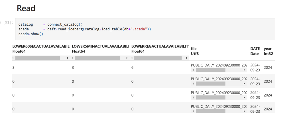
My initial plan was to use Daft for data preparation as it has a good integration with Iceberg catalog, unfortunately as of today, it does not support adding filename as a column in the table destination, so I endup using Duckdb for data preparation and Daft for reading from the catalog.

Daft added support for adding filename when reading from csv, so, it is used both for reading and writing.

The convenience of the catalog

what I really like about the catalog is the ease of use, you just need to initiate the catalog connection once.

def connect_catalog():
      catalog = SqlCatalog(
      "default",
      **{
          "uri"                : postgresql_db,
          "adlfs.account-name" : account_name ,
          "adlfs.account-key"  : AZURE_STORAGE_ACCOUNT_KEY,
          "adlfs.tenant-id"    : azure_storage_tenant_id,
          "py-io-impl"         : "pyiceberg.io.fsspec.FsspecFileIO",
          "legacy-current-snapshot-id": True
      },
                        )
      return catalog 

The writing is just one line of code, you don’t need to configure storage again

For writing , you just use something like this

catalog.create_table_if_not_exists('tbl', schema=df.schema, location=table_location + f'/{db}/{tbl}')
catalog.load_table(f'{db}.{tbl}').append(df)