Iceberg on a single node is coming together

For a long time, whenever I tried to use Iceberg outside the JVM ecosystem, something I needed seemed to be waiting for the next release. It took longer than I hoped, but lately I have been able to get much further with the engines I use.

chDB can authenticate to OneLake with a token, Polars now runs all 22 queries in this benchmark, and DuckDB’s cache feels like absolute magic on the second pass. I still ran into bugs, but I could run both reads and writes across several engines against the same Iceberg catalog.

I took two of my notebooks and port them to GitHub Actions as python script across DuckDB, Polars, chDB, LakeSail, Spark and Daft. One runs analytical queries; the other reads CSVs and writes Iceberg tables. I wanted to see how each handled the workloads on a small 4-core runner.

The data lives in OneLake. Reading through its Iceberg REST catalog is already available; the write support I used is still in private preview.

Both benchmarks run on a public 4 vCPU / 16 GB runner. The engines connect to the catalog either directly or through pyiceberg. OIDC federation provides a token per job, so there is no client secret to store. The same approach should work with other Iceberg REST catalogs, provided the engine supports their storage and authentication.

The code, the raw JSON of every run and the charts are in djouallah/lakehouse_benchmark.

Reading: TPC-H-like queries at SF10

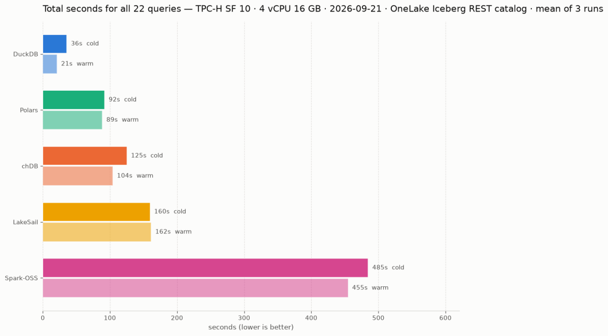
The tables are generated with tpchgen, uploaded as Parquet and registered with pyiceberg’s add_files. DuckDB and LakeSail could have written them just fine, but I wanted to stay neutral. Each engine attaches the catalog, runs the 22 queries, then runs the same 22 again immediately. Those are the cold and warm passes below; catalog attach time is excluded. The chart and the table are the mean of three runs on 20 and 21 September 2026. This is a small single-node comparison, not an official TPC-H benchmark.
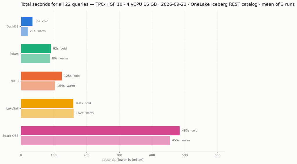
EngineVersionColdWarm
DuckDB2.0.0 dev35.9s21.3s
Polars2.0.0-rc.292.1s88.6s
chDB4.4.0125.4s104.5s
LakeSail0.7.1159.9s161.6s
Spark-OSS4.1.3484.9s454.9s

Spark open source, not to be confused with Fabric Spark, is a single-node JVM on 4 cores here. Thanks to AI, running Spark locally is no longer a scary experience. Unfortunately Daft is missing: at 0.7.25 it runs 16 of the 22 queries, because l_extendedprice * (1 - l_discount) overflows its decimal precision ceiling of 38 (Daft#7532). I like Daft and would love to include it in the full query comparison once this is fixed. It does complete the ETL workload below.

Writing: Light ETL

1000 daily AEMO CSV files, 52 GB, are landed once in the lakehouse Files/ section. Each engine reads all of them, filters, casts and writes one Iceberg table of 149,146,763 rows through the same catalog. DuckDB, LakeSail and Spark have their own Iceberg writer. chDB and Polars stream Arrow batches into pyiceberg. Daft has its own writer over a pyiceberg table.
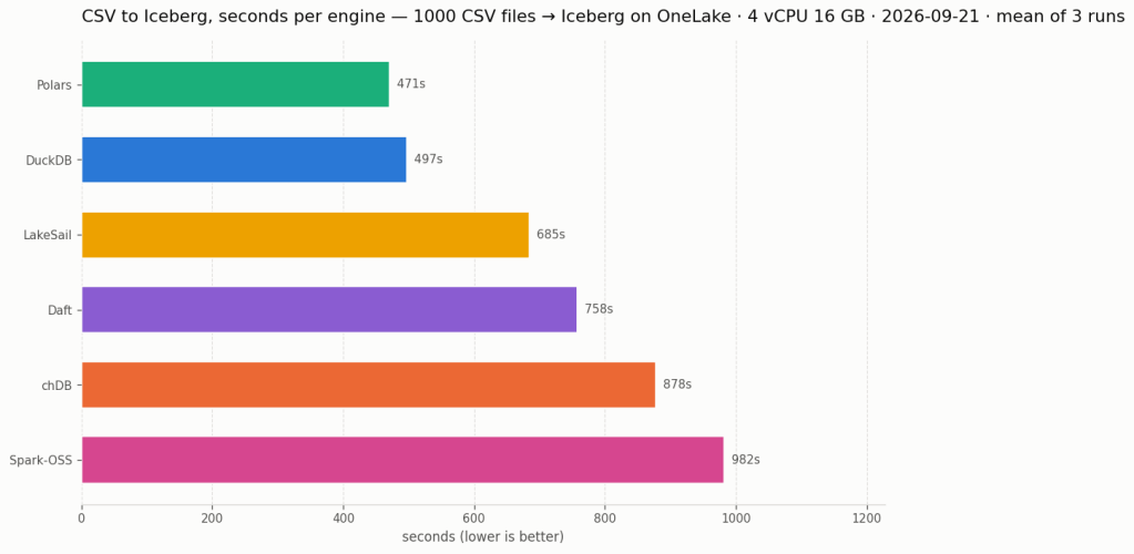
EngineLoad
Polars470.8s
DuckDB497.4s
LakeSail684.5s
Daft757.9s
chDB878.1s
Spark-OSS982.2s

Every engine ends with the same row count. Load time includes recreating the table, reading the CSVs, transforming, writing and committing; session setup and catalog attach are timed separately. There is one load pass per engine, and the chart and the table are the mean of three runs. Snapshot isolation and concurrent writes will have to wait for another blog. The Iceberg write path used here is in private preview.

Random learnings, in no particular order

  • DuckDB needed AZURE_TRANSPORT_OPTION_TYPE=curl on this Linux runner. Without it the Iceberg attach succeeds and every data-file read fails with a message that looks exactly like a missing credential. Setting the transport fixed it. I had not seen this in the Fabric notebook.
  • chDB returned 41 rows for Q13, everybody else 42. ClickHouse defaults join_use_nulls=0 and fills unmatched outer-join cells with default values instead of NULL. The row-count smoke test caught this, and the benchmark now sets join_use_nulls=1.
  • The catalog cache settings do not all mean the same thing. I configured a 15-minute lifetime, but LakeSail’s “table cache” caches the table listing, not the loaded table. It still loads table metadata on every statement, adding REST requests even on the warm pass (sail#2629).
  • Daft’s six query failures come from decimal arithmetic. CTEs, EXISTS and correlated subqueries all work. It also rejects backticks outright, which looked like a total dialect failure until I read the error. Separately, its Azure URI parser drops the container on OneLake hosts; the bench works around it with az:// paths. The proposed fix is Daft#7533.
  • Nothing is partitioned, on purpose. The pyiceberg streaming append used here only supports unpartitioned tables. A first version that materialised batches to partition by year took the 16 GB runner down at 100 files. So every engine writes the same unpartitioned shape and year stays a plain column.

Spark, and why it has no native accelerator here

Spark-OSS is 4.1.3 with Iceberg 1.11 and hadoop-azure 3.4.2. I also looked at Comet and Gluten/Velox, but could not use either for this benchmark.

  • Comet supports Spark 4.1 and ships a native Iceberg reader, but its readable schemes are file, s3, s3a, gs, oss. An abfss table is declined at planning time and runs on the JVM as if the plugin were not there. I left Comet out because it could not accelerate these scans. Filed as datafusion-comet#6058.
  • Gluten/Velox has a Velox ABFS connector, but I could not find a published package for Spark 4.x to test (This basically what Fabric NEE uses)

Conclusion

All six engines completed the CSV-to-Iceberg load. Five completed all 22 read queries; Daft completed 16. Being able to try this many engines against one catalog, with the data staying in OneLake, is what I find exciting. chDB’s token support and Polars running all 22 SQL queries give me more options for the notebooks I already use.

DuckDB was fastest on the reads, and on the load it traded first place with Polars from run to run. DuckDB’s read total fell from 36s to 21s on the second pass, about 40%. The other engines improved less, and LakeSail’s warm pass came out slightly slower than its cold one. That makes repeated reads worth testing separately from a one-pass load. It does not tell us exactly what each engine cached or how many bytes it fetched; chDB also has a filesystem cache configured here.

For my ETL workload, the cache does not matter: read the new files, transform them and write the table.

If you want to see how much things have changed, have a look at these TPC-H SF10 results from four years ago.

Note: The write benchmark requires access to the private preview used here coming soon.
Writing Databricks Parquet That VertiPaq Likes

This post, the repo and every number in it are personal opinion. Nothing here is a Fabric position, benchmark or recommendation.

My colleague Eiki published a post on Microsoft’s white paper on Power BI architecture choices for Azure Databricks. Read it first: it covers the four storage modes, the headline findings, and links to the paper. I assume you know what the paper measured.

I like the paper for a different reason. It benchmarks a lakehouse as designed: open files on object storage, one vendor writes, another reads, Parquet is the only contract. Such benchmarks are rare, hard to reproduce and usually opinionated. This one is deliberately neutral (maybe too neutral) , The dataset is so uniform that V-Order has little room to differentiate the writers, so all writers start on relatively equal ground.

I have written before about VertiPaq reading Parquet that other engines wrote: Optimizing Parquet Layout for Power BI Direct Lake Mode (Dec 2024), Just VOrder, don’t try to understand how VertiPaq works (Nov 2025) and Writing Parquet That VertiPaq Likes (Aug 2026).

The short version: VertiPaq reads Parquet from any producer. It does not need V-Order. It prefers a layout it can transcode fast and hold small, and V-Order is one way to produce it.

This post applies that idea to Spark on Databricks. I am not a Spark expert; I know delta-rs much better. The Parquet concepts carry over, the knobs do not, and Databricks has many settings that interact.

AI helped me navigate them. Where the repo gets Spark wrong, the mistake is mine. Corrections welcome.

What I did

The paper tunes the Databricks write with the mainstream, documented settings, as an industry paper has to. This is a personal blog, so I can be less orthodox and go low level 🙂 I tried a few little-known knobs instead.

All of them are cluster configuration for row-group size and dictionary encoding, the same lines for every table, plus one optional step per fact table: a single clustering key on the column the reports filter on (nothing fancy it is just a global sort).

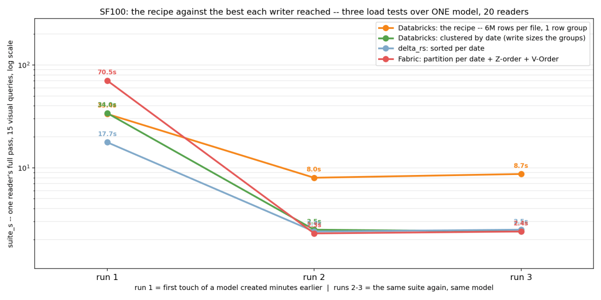
I used the paper’s protocol: TPC-DS at SF100 and SF1000, its DAX capture, 20 concurrent readers, three load tests back to back on one model. Two changes: the semantic model is deleted after the three runs so the next run starts cold, and the OneLake cache is on because my Databricks tenant is in another region. Only the very first run at a scale factor reads across regions; every later run 1 reads from the cache, so it measures the transcode alone.

Note: I used Fabric layout as it is.

Databricks writes, Direct Lake reads through the mirrored catalog. The configuration, what each line does and what breaks it are in the repo. This post is results only.

The results

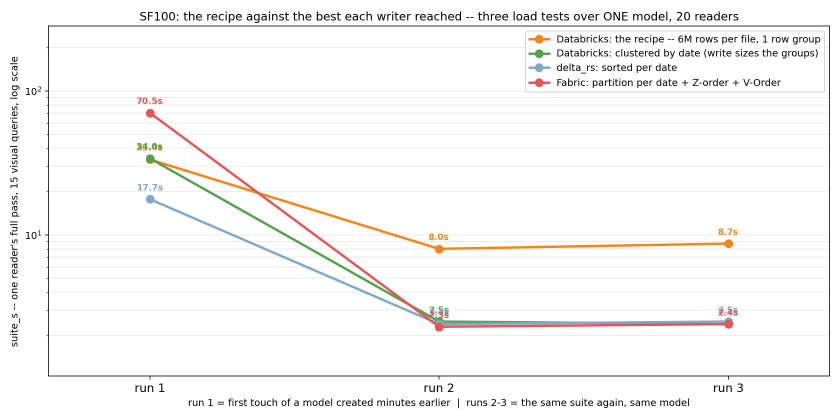
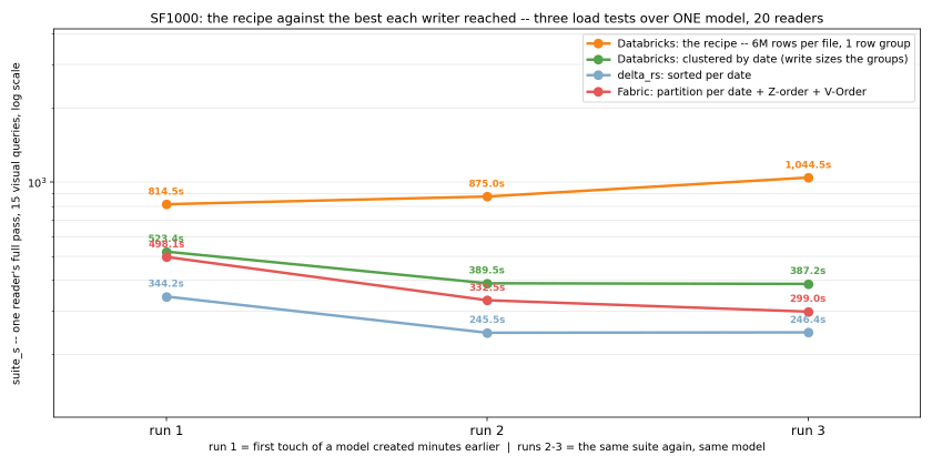
Each chart shows the configuration alone, the configuration with the clustering key, and the best layout of each other writer: delta-rs sorted on the date key, and the paper’s Fabric layout of one partition per date with Z-order and V-Order.

Run 1 pays the transcode; runs 2 and 3 rerun the same queries on the loaded model.

At SF100, the configuration alone produces dictionary encoding and large row groups, but is about three times slower than every ordered layout. Adding the clustering key on the date matches the paper’s V-Order layout, with row groups more than ten times larger.

At SF1000, the configuration alone never really warms up: each run is slower than the last, while the three ordered layouts do. That is why the clustering key is not just an optimisation in the recipe; it is what makes the layout usable at this scale. The clustered arm still trails delta-rs and the paper’s layout at SF1000: the clustering did not fully sort the rows at that scale, and the repo carries that as open. Why delta-rs has the best cold run at both scale factors is still a mystery to me.

The interesting part is that VertiPaq does not care who wrote the Parquet. It cares about the physical layout it has to transcode.

The repo

github.com/djouallah/parquet_layout_vertipaq_spark has the configuration, the clustering step, what undoes it, the numbers behind both charts and what is still open.

It also ships a Claude Code skill that applies the recipe.

Some observations on single node vs distributed systems. 

Was doing an experimentation in a Fabric notebook, running TPCH benchmarks and kept increasing the size from 1 GB to 1 TB, using Spark, DuckDB reading both parquet files and native format,  it is not a very rigorous test, I was more interested about the overall system behavior then specific numbers, and again benchmarks means nothing, the only thing that matter is the actual workload.

The notebook cluster has 1 driver and up to 9 executors, spark dynamically add and remove executors , DuckDB is a single node system and runs only inside the driver.

Some observations

  • When the data fits into one machine, it will run faster than a distributed system, (assuming the engines have the same performance), in this test up to 100 GB , DuckDB Parquet is faster than Spark.
  • It is clear that DuckDB is optimized for its native file format, and there are a lot of opportunities to improve Parquet performance.
  • At 700 GB, DuckDB native file  is still competitive with Spark, even with multiple nodes, that’s very interesting technical achievement, although not very useful in Fabric ecosystem as only DuckDB can read it.
  • At 1 TB, DuckDB parquet timeout and the performance of the native file format degraded significantly, it is an indication we need a bigger machine.  

Although clearly I am a DuckDB fan, I appreciate the dynamic allocation of Spark resources,Spark is popular for reason 🙂

Yes I could have used a bigger machine for DuckDB, but that’s a manual process and does changes based on the specific workload, one can imagine a world where a single node get resources dynamically based on the workload.

I think the main takeaway, if a workload fits into a single machine then that will give you the best performance you can get.

Edit : to be clear, so far the main use case for Something like DuckDB inside Fabric is cheap ETL, I use it for more than a year and it works great, specially with the fact that single node notebooks in Fabric start in less than 10 seconds.

What is the Fastest Engine to sort small Data in a Fabric Notebook?

TL;DR : using Fabric Python Notebook to Sort and Save  Parquet files  up to 100 GB shows that DuckDB is very competitive compared to Spark even when using Only half the resources available in a compute pool.

Introduction : 

In Fabric the minimum Spark compute that you can provision is 2 nodes, 1 Driver and 1 Executor,  my understanding, and I am not an expert by any means is : Driver Plan the Work and Executor do the actual Works, but if you run any no Spark code, it will run in the driver, basically DuckDB use only the driver, the executor is just sitting there and you pay for it.

The experiment is basically : generate the Table Lineitem from the TPCH dataset as a folder of parquet files and sort it on a date field then save it. Pre-sorting the data on a field used for filtering is a very well known technique.

Create a Workspace

When doing POC, it is always better to start in a new workspace, at the end you can delete it and it will remove all the artifacts inside it. Use any name you want.

Create a Lakehouse

Click New then Lakehouse, choose any name

You will get an empty lakehouse (it is a just a storage bucket with two folders, Files and Table)

Load the Python Code

The Notebook is straightforward, Install DuckDB , create the data files if they don’t exist already, sort and save in a delta table using both DuckDB and Spark

Define Spark Pool Size

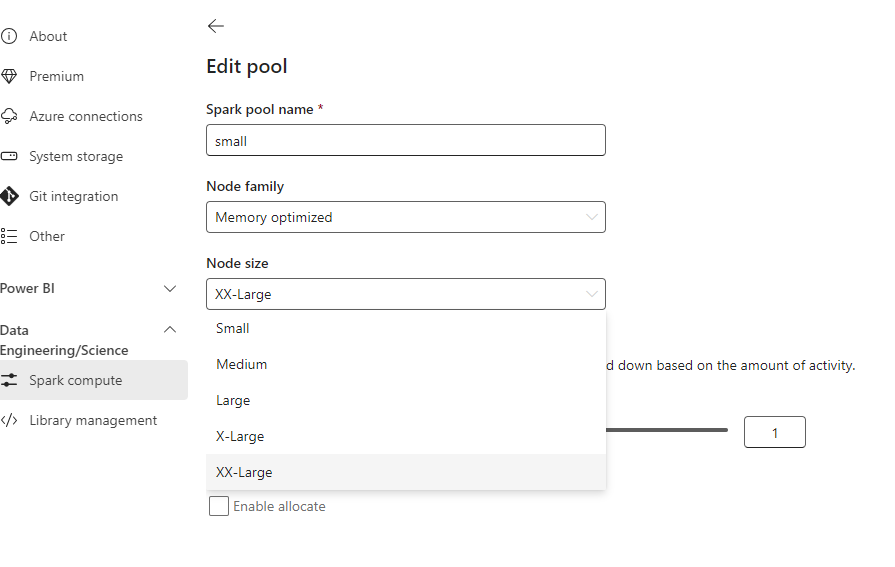
By default the notebook came with a starter pool that are warm and ready to be used, the startup is in my experience is always less than 10 second, but it is a managed service and I can’t control the number of nodes, instead we will use custom pool where you can choose the size of the compute and the number of nodes in our case 1 driver and 1 executor,  the startup is not bad at all, it is consistently less than 3 minute.

Schedule the Notebook

I don’t not know, how to pass a parameter to change the initial value in the pipeline, so I run it using a random number generator`, I am sure there is a better way, but anyway, it does works, and every insert the results

The Results

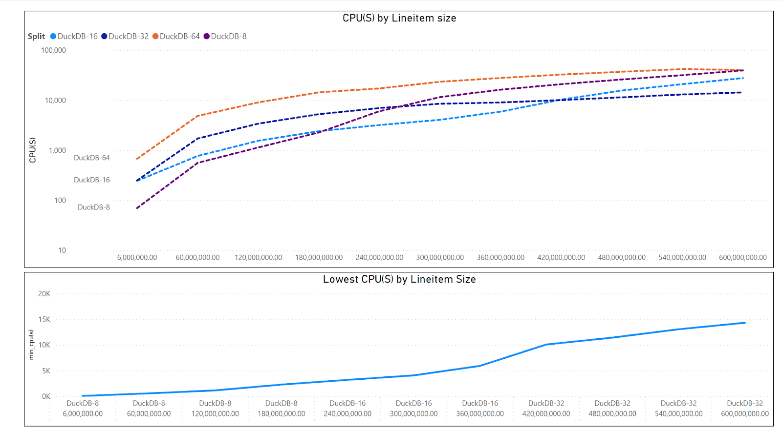
The Charts  show the resource usage by data size, CPU(s) =  Duration * Number of cores * 2.

Up to 300 Million rows, DuckDB is more efficient even when it is using only half the resources. 

To make it clearer , I build another chart that show the Engine combination with less resource utilization by Lintem size

From 360 Million rows, Spark became more economical ( with the caveat that DuckDB is just using half the resources) or maybe DuckDB is not using the whole 32 cores ?

Let’s filter only DuckDB

DuckDB using 64 cores is not very efficient for the size of this Data.

Partying Thoughts

  • Adding more resources to a problem does not make it necessarily an optimal solution, you get faster duration but it costs way more.
  • DuckDB Performance even using half the compute is very intriguing !!!
  •  Fabric Custom pools are a very fine solution, waiting around 2 minutes is worth it.
  • I am no Spark expert, but it will be handy to be able to configure at runtime a smaller Executor compute, in that case, DuckDB will be cheaper option for all sizes up to 100 GB and maybe more.