I like the paper for a different reason. It benchmarks a lakehouse as designed: open files on object storage, one vendor writes, another reads, Parquet is the only contract. Such benchmarks are rare, hard to reproduce and usually opinionated. This one is deliberately neutral (maybe too neutral) , The dataset is so uniform that V-Order has little room to differentiate the writers, so all writers start on relatively equal ground.
The short version: VertiPaq reads Parquet from any producer. It does not need V-Order. It prefers a layout it can transcode fast and hold small, and V-Order is one way to produce it.
This post applies that idea to Spark on Databricks. I am not a Spark expert; I know delta-rs much better. The Parquet concepts carry over, the knobs do not, and Databricks has many settings that interact.
AI helped me navigate them. Where the repo gets Spark wrong, the mistake is mine. Corrections welcome.
What I did
The paper tunes the Databricks write with the mainstream, documented settings, as an industry paper has to. This is a personal blog, so I can be less orthodox and go low level 🙂 I tried a few little-known knobs instead.
All of them are cluster configuration for row-group size and dictionary encoding, the same lines for every table, plus one optional step per fact table: a single clustering key on the column the reports filter on (nothing fancy it is just a global sort).
I used the paper’s protocol: TPC-DS at SF100 and SF1000, its DAX capture, 20 concurrent readers, three load tests back to back on one model. Two changes: the semantic model is deleted after the three runs so the next run starts cold, and the OneLake cache is on because my Databricks tenant is in another region. Only the very first run at a scale factor reads across regions; every later run 1 reads from the cache, so it measures the transcode alone.
Note: I used Fabric layout as it is.
Databricks writes, Direct Lake reads through the mirrored catalog. The configuration, what each line does and what breaks it are in the repo. This post is results only.
The results
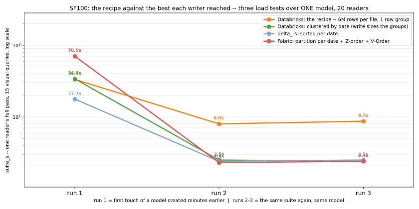
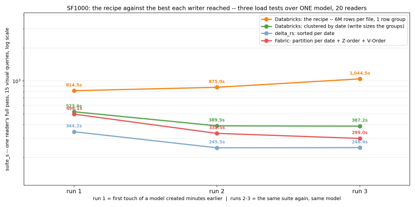
Each chart shows the configuration alone, the configuration with the clustering key, and the best layout of each other writer: delta-rs sorted on the date key, and the paper’s Fabric layout of one partition per date with Z-order and V-Order.
Run 1 pays the transcode; runs 2 and 3 rerun the same queries on the loaded model.
At SF100, the configuration alone produces dictionary encoding and large row groups, but is about three times slower than every ordered layout. Adding the clustering key on the date matches the paper’s V-Order layout, with row groups more than ten times larger.
At SF1000, the configuration alone never really warms up: each run is slower than the last, while the three ordered layouts do. That is why the clustering key is not just an optimisation in the recipe; it is what makes the layout usable at this scale. The clustered arm still trails delta-rs and the paper’s layout at SF1000: the clustering did not fully sort the rows at that scale, and the repo carries that as open. Why delta-rs has the best cold run at both scale factors is still a mystery to me.
The interesting part is that VertiPaq does not care who wrote the Parquet. It cares about the physical layout it has to transcode.
This rabbit hole started with a simple observation: VertiPaq seemed to like parquet produced by delta-rs more than parquet produced by DuckDB — and that drove me nuts. delta-rs was at the time a niche library for nerds; Fabric didn’t even have a Python notebook. The mental model was simple: write with Spark, get V-Order, get the best possible layout for Power BI.
It is 2026; Fabric is more widespread, and there are simply more patterns and use cases:
New Fabric workspaces default Spark to the writeHeavy resource profile, which does not write V-Order.
Customers — especially on smaller SKUs — routinely write with delta-rs from Python notebooks.
Reading tables written by Snowflake, Databricks and BigQuery through Direct Lake is a production pattern.
So “what parquet is friendly to Vertipaq” is now a legitimate data engineering question — I can’t tell you how happy I was when I read this tweet 🙂
The short version
Row groups of a few million rows : 2–6M rows per group; never go above 16M, VertiPaq’s segment ceiling.
Dictionary-encode every column — and make the file footer say so.
One global ORDER BY, lowest-cardinality columns first, date up front. No clustering, no Z-ordering, none of that.
Delta vs Iceberg does not matter. Only the parquet inside the table matters.
Method
I treated VertiPaq as a black box and did what experimental science does with a phenomenon it doesn’t understand: change one variable, measure, repeat. Nothing here is confidential or internal — every number was measured from the outside, on tables anyone can rebuild.
One more thing changed this year: AI became genuinely useful for this kind of work, because it never gets bored. Sweeping writers × row-group sizes × file sizes × sort orders across hundreds of runs is exactly the tedium it doesn’t feel.
Two experiments.
First: figure out why VertiPaq preferred delta-rs output.
Second: run multiple writers and vary row-group count, file size and ordering, measuring cold, warm and hot query cost.
Caveat. Hot behaviour is well documented — after all, it is the same in-memory format as import mode — so I am more interested in cold runs (first touch of a fresh model), even though most real-world traffic is hot: a live model transcodes once and then serves from RAM.
The datasets are rather smallish — the biggest table here is around 600M rows. As a data analyst I have always dealt with small data, so I am optimising for the workload I actually care about.
How Direct Lake reads your parquet
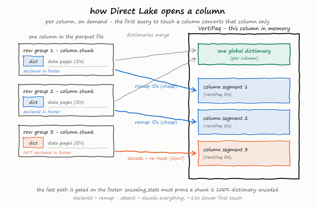
The mechanism that explains almost every finding. Transcoding is per column, on demand: the first DAX query to touch a column that is not yet in memory converts that column only into VertiPaq’s in-memory format. The column’s per-row-group parquet dictionaries are merged into one global VertiPaq dictionary, and each row group of the column is loaded as one resident column segment, remapping parquet data IDs onto VertiPaq IDs on the way in. Every query after that scans the segments the transcode produced. Query latency — and capacity consumption — is therefore a property of how the parquet was written.
Findings
Dictionary encoding is the big one
VertiPaq is itself a dictionary-based engine. When a chunk arrives dictionary-encoded, the transcode merges the parquet dictionary into the column’s global one and remaps the data IDs — it never decodes the values. Anything else has to be decoded and re-hashed, value by value, at load time. On a single 144M-row DECIMAL(18,4) column, PLAIN measured 618.6 MB against 423.1 MB dictionary-encoded — ~200 MB extra and a re-encode, on one column.
The surprise is that the encoding alone isn’t enough: the declaration is part of the encoding. The engine takes the cheap remap path only when the footer’s encoding_stats prove a chunk is entirely dictionary-encoded without decoding its pages. DuckDB’s writer emitted no encoding_stats at all until duckdb#24957 (merged 2026-08-24, currently in main only). That PR measures the cold first-touch of a 142M-row dictionary string column falling from 10,857.5 ms to 689.3 ms — about 15×, with identical pages. The attribution was verified the hard way: synthesising only that footer field into an otherwise unmodified file reproduces the speedup. A second PR, duckdb#24645 (merged 2026-08-10), adds a data_page_size_limit option — before it, DuckDB often wrote one huge data page per column chunk.
Row-group size: a tension between cold and hot
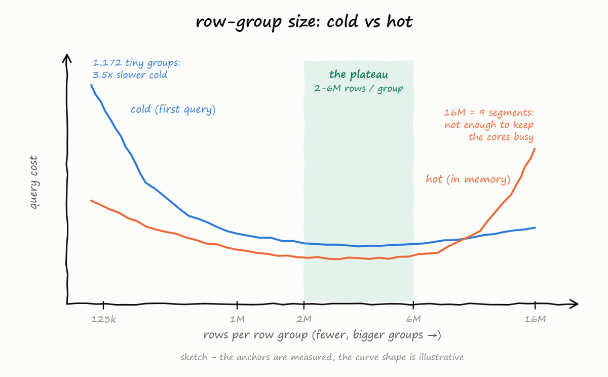
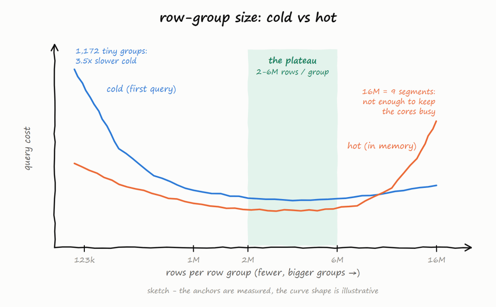
There is no single best size, but both ends fail measurably. Every row group is one more dictionary merge and one more segment to set up per column, which is why tiny groups murder the cold tier: the same DuckDB in the same notebook was 3.5× slower cold (96,503 ms vs 27,785 ms) when a library default sliced a 144M-row table into 1,172 groups of ~123k rows. At the other end, 16M rows — VertiPaq’s segment ceiling — was the worst sorted geometry measured: nine segments starve the scan pool. Cold prefers slightly bigger groups than hot, but very big groups are bad for both.
Power BI doesn’t disclose how many cores it uses, so the practical rule is: enough row groups to keep the cores busy. On the 144M-row table, warm query time stepped down between 19 and 24 groups (≈5,700 ms → 3,221 ms), and 72 groups bought nothing over 24. Hence the plateau: 2–6M rows per group.
A global sort keeps paying after the data is in memory
Transcoding does not change row order — it is essentially a working data copy into memory. So a sort applied at write time survives into the resident segments, which is why ordering matters for hot runs too, not just for compression.
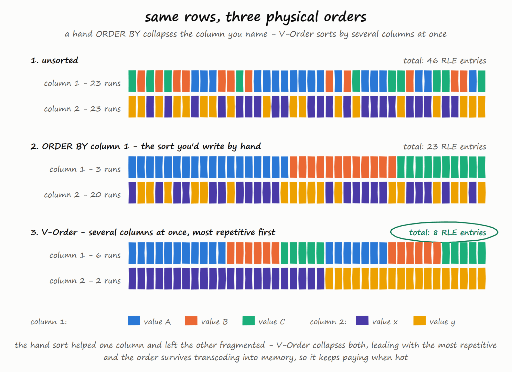
A single global ORDER BY with low-cardinality columns first (and a preference for date) produces long RLE runs. It is not V-Order — but in some cases it is good enough. When V-Order does engage, what it’s worth depends on the surface — column count × categorical skew — not row count: on a skewed 17-column taxi table it collapsed the most repetitive column to 3,371× fewer runs; on a near-unique 5-column table it left row order untouched and still shrank files 16%. One caution from the sweep: an alternative sort key cut file size a further 30% and bought statistically zero query time — sort for the columns your queries filter on, not for size on disk.
This is also the cleanest way to see what V-Order’s reorder actually is. A hand-written ORDER BY collapses the column you name and leaves the others fragmented; V-Order sorts by several columns at once, most repetitive first — the taxi measurement above is its signature, runs falling off exactly as an encoding-driven sort predicts.
VertiPaq doesn’t like ragged row groups
delta-rs closes a file the moment the size cap is hit, truncating the in-progress row group — measured writing groups at 0.43× their declared rows. A truncated group isn’t just small; it makes segment sizes uneven, exactly the non-uniform scan load you were sizing row groups to avoid. I’ve proposed a fix in delta-rs#4677 — still open, and opt-in — which rolls files only on row-group boundaries.
Dynamic row group size at write time are very hard.
I built a personal package, duckrun, using delta-rs and DuckDB and tried a clever optimisation. The plan: before writing a query’s result, estimate its row count and compute the perfect row-group size on a 1M–16M scale. It failed completely, because query planners are bad at estimating output size — DuckDB estimated ~14.9M rows for a table that actually held 143,980,961, 9.7× too low — so the “optimised” geometry was off by an order of magnitude. Derive geometry from an exact count (the table you’re rewriting, the Delta log) — never from an estimate. Not only that: in an initial version the cost of the estimation was nearly the same as writing the table 🙂
Anyway, I endup writing 6M as the default row group everywhere, i feel it is a good enough compromise
Takeaway
V-Order is usually understood as row reordering — and the reordering is real; the hard part is not the reordering itself but doing it fast (that’s the secret sauce basically), to be super clear, V-order is a local sort, not global
But it is not only that: a V-Order write also sets the row-group geometry and runs the encoding pass, keeping a declared dictionary on every column.
Two consequences follow:
If you write with a Fabric engine, turning V-Order on is a no-brainer, and honestly, it should be the default in my personal opinion.
measured here at ~8% of build compute for up to 2.8× less query capacity (1,332 vs 3,769 CU on identical data) — the write premium is paid once, while queries pay every day. I do wish it were simpler to turn on: changing the Spark write profile is not obvious, and a lot of users don’t even know it is there. As someone who used VertiPaq for more than a decade with zero knowledge of columnar data structures, I suspect there must be a better way.
If you write with anything else — Snowflake, Databricks, delta-rs, DuckDB — my hope is that there will be more public specifications on how to optimize parquet layout for VertiPaq.
Thanks to Krystian Sakowski for answering my silly questions 🙂
duckrun is a package I built using AI exclusively, to solve pain points I hit when using Fabric Python notebooks. I like DuckDB very much, but I was tired of manually discovering table names every time and writing long Python deltalake code just to write a Delta table, so I combined those two packages under one helper package to make my workflow smoother. Recently I discovered how awesome dbt is, so why not add a dbt adapter too. Then someone trolled me about the lack of snapshot isolation when doing read-modify-write on the same table. Luckily DuckDB now exposes the read version in delta_scan (before, you had to do the weird attach thing), so I have something that might actually be useful. The rest of the blog is written by AI. It wrote my code, so I don’t see the issue; it’ll even write my blog.
I also added a web page with some projects I built: dbt projects I ported, and some non-trivial SQL statements with proper snapshot isolation.
So yes, it’s a hack, until Iceberg matures or we get a better Delta write story in DuckDB.
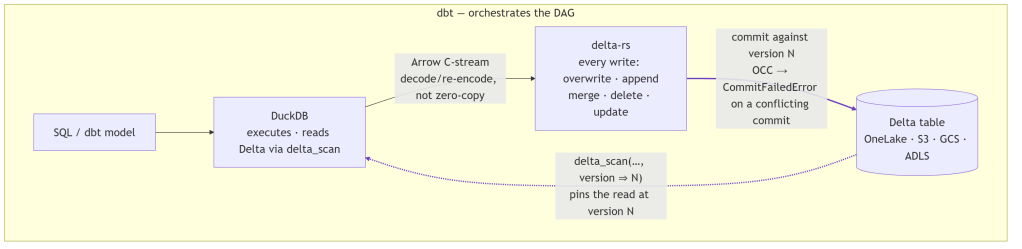
At its core, duckrun is a four-part split: DuckDB executes the SQL, Arrow streams the result, delta-rs commits it to Delta, and dbt (optionally) orchestrates the whole DAG.
It’s storage-agnostic, running anywhere DuckDB and delta-rs can reach: local filesystem, S3, GCS, ADLS, OneLake. In practice I test it on the local filesystem and Microsoft Fabric OneLake. S3 and GCS use the same code path, but I barely touch them, so treat them as untested.
The gap it fills
DuckDB reads Delta well (delta_scan). It does not write it well: its Delta support is blind INSERT only (no UPDATE, DELETE, or MERGE), and its trajectory points at writing through Unity Catalog, which defeats the point of filesystem-native Delta. So if you want DuckDB’s engine but need upserts on Delta tables, there is no single tool that does both today.
Approach
Reads Delta
Writes Delta (merge/update/delete)
DuckDB SQL engine
DuckDB alone
✅
❌ (blind INSERT only)
✅
delta-rs alone
✅
✅
❌
duckrun
✅
✅
✅
duckrun’s answer is a split:
DuckDB runs all SQL and model logic, and reads Delta through delta_scan views.
delta-rs handles every write: overwrite, append, merge, delete, update.
Arrow bridges the two: a DuckDB relation is streamed to delta-rs over the C-stream interface.
Snapshot isolation ties it together: each read pins a Delta version, and each read-modify-write commits against the version it read, so a concurrent commit errors instead of silently clobbering.
That’s the whole architecture. The README calls it glue, and that’s accurate: each layer does only the one thing it’s set up to do.
Two costs come with this. Two engines split one RAM budget with no shared allocator, and the Arrow handoff isn’t zero-copy: DuckDB’s native vector format isn’t Arrow, so each batch is decoded and re-encoded as it streams across the Arrow C Data Interface (a batch-at-a-time ArrowArrayStream, so even a large write never fully materializes in memory). duckrun manages this with a cgroup-aware memory split, sampled per job so it doesn’t get OOM-killed on Fabric/k8s, where DuckDB otherwise sees the whole node. The fractions are of the effective limit: on a merge, 0.3 to DuckDB and 0.6 to delta-rs spill, leaving 0.1 slack; on a plain write, 0.85 to DuckDB. The split leans toward delta-rs because that’s where the memory goes: profiling a merge attributes ~99% of resident memory to delta-rs and only ~15 MB to DuckDB. Keeping every write behind delta-rs also means the bridge (and the memory juggling) can be deleted the day DuckDB ships a real Delta writer, without touching the read or state model.
connect: read first
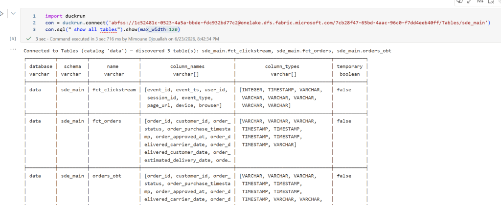
connect() is read-only by default, so you can point it at a lakehouse and explore with no chance of an accidental write. Tables are discovered for you, with no manual name bookkeeping:
Attach more lakehouses and query across them by three-part name. This is where the data warehouse case shows up: in Fabric a Warehouse is just a write-locked Lakehouse, so you attach it read_only=True next to a writable Lakehouse and join the two:
conn.sql accepts CREATE [OR REPLACE] TABLE AS, INSERT, UPDATE, DELETE, ALTER … ADD COLUMN, MERGE, and DROP (a soft tombstone: delta-rs has no drop, so data files persist until you purge them). CREATE TEMP TABLE and CREATE VIEW stay native DuckDB. Things that can’t be honored cleanly, like multi-statement strings or UPDATE … FROM, are rejected rather than silently mishandled.
The surface is small. It mirrors the Delta/DeltaTable API so notebook code reads familiarly, but there is no fluent transform builder and no second SQL engine. Transforms are SQL, run by DuckDB.
Snapshot isolation
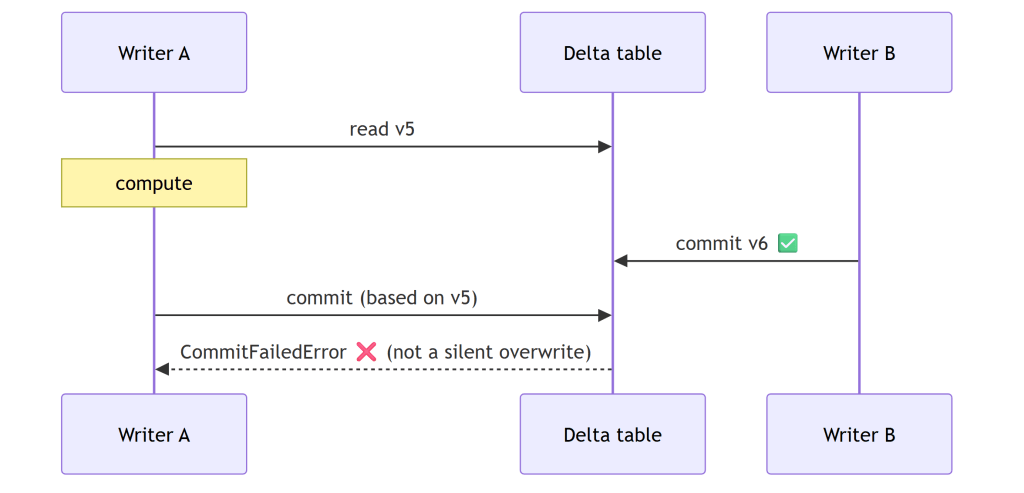
This started as someone trolling the project over read-modify-write on the same table, and it turned into the guarantee I rely on most. Honestly, I come from a Dataflow Gen1 background (basically a single writer), so all this concurrency stuff never made much sense to me. In a Lakehouse, where anyone can write to a table, even accidentally, it suddenly becomes a real factor. (Thanks Raki for the harsh feedback, lol.) A lakehouse has no transaction manager and no single-writer guarantee: two pipelines, a double-fired job, or a notebook racing a scheduled run can all commit to the same table. The dangerous shape is read → compute → write: if someone commits in between, a naïve write at HEAD silently overwrites them, a lost update with no error. duckrun’s job is to turn that into a CommitFailedError.
What’s fenced, and what isn’t.delete, update, and merge are read-modify-writes (they read the current rows, compute a change, then commit), so duckrun pins each to the version it read and delta-rs’s OCC validates the commit over (read, HEAD]. A conflicting concurrent commit makes them fail. Plain append and overwrite are not fenced, by design: they match Spark’s SaveMode. An append rebases onto HEAD (appends don’t conflict), and an overwrite is last-writer-wins. So the fence is automatic exactly where a lost update is possible, and absent where it isn’t.
How the OCC works. There’s no lock manager anywhere. A Delta commit is the atomic creation of the next log entry, _delta_log/…{N+1}.json, so if a racing writer already wrote it, your put-if-absent loses and delta-rs raises CommitFailedError. Optimistic, filesystem-native, no coordinator. The gap OCC alone leaves: it only checks the commit instant, not the version you read.
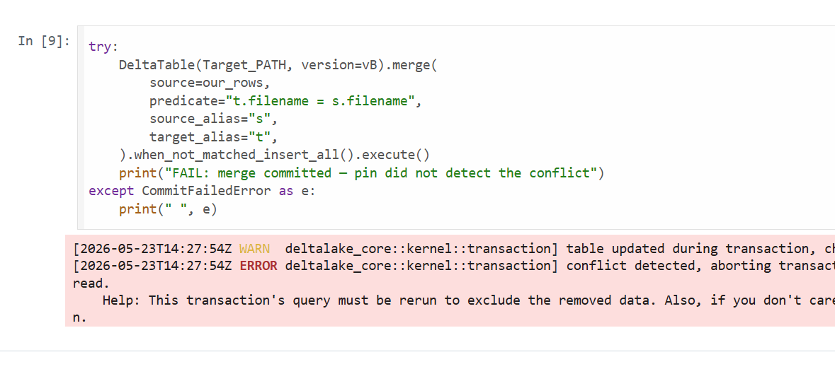
Pinning the version you read, the same whether you write SQL or a DataFrame. A DeltaTable handle captures the version at forName() (call it vB), and every merge() / delete() / update() through it commits against vB, so OCC validates the whole (vB, HEAD] window, not just the instant of the commit. conn.sql("delete …" / "update …" / "merge …") funnels into the exact same engine path, pinned the same way: there is no second code path for SQL. And DuckDB exposing the read version in delta_scan(…, version => vB) (the reason for the duckdb >= 1.5.4 floor) lets the read sit on vB too, so a read-modify-write split across statements still lands on one snapshot. Spark/Delta fences only the commit instant; this fences the version you actually read.
append_if_unchanged / overwrite_if_unchanged are the fenced siblings of plain append/overwrite. I had to coin the terms, because Delta/Spark has no built-in fenced append (you’d hand-write a MERGE for it). They’re a version compare-and-swap: load the table at the version you read and pass max_commit_retries=0 so delta-rs won’t rebase. If anything committed since, the target version is already taken and the commit fails. For the watermark/idempotent-append case this is cheaper than a merge, with no target scan and no key join. (safeappend is the deprecated alias.)
The dbt adapter
A thin wrapper over dbt-duckdb that adds Delta-backed table and incremental materializations; everything else (views, seeds, sources, tests, plugins) is inherited. Point a profile at a lakehouse and dbt run:
dbt with no catalog. Normally dbt leans on a metastore to know what exists and to resolve {{ this }}, ref(), and is_incremental(); duckrun has none, and state still survives across separate dbt build processes. At run start the adapter discovers Delta tables on disk (glob for local/az/s3/gs; the OneLake DFS REST API for abfss, since DuckDB can’t glob it reliably) and registers each as a delta_scan view named to match dbt’s database.schema.identifier. That view is what makes those references resolve against real Delta tables. Each materialization pre-registers its own {{ this }} view before running, then recreates the view after the delta-rs write, since that write lands a new Delta version and the old view would otherwise point at stale files. The namespace is rebuilt from storage on every run instead of read from a catalog.
Incremental strategies:
Strategy
Behavior
merge (default with unique_key)
upsert
insert
insert new keys only
append (default without unique_key)
blind append
append_if_unchanged / safeappend
append, commit only if version unchanged: cheap, no target scan, errors on conflict
microbatch
delete+insert per event_time window
Compaction and 7-day vacuum run automatically (every run for overwrites; past a file-count threshold for incrementals).
Two limits worth knowing up front. First, writes are single-threaded within a run (in-process delta-rs isn’t thread-safe; cross-process concurrency is fully supported). Second, constraints are enforced at the write boundary, not stored in the table: a contract with not_null columns is checked by a guard query before the write, so a null fails with NOT NULL constraint failed and the prior Delta version is left untouched. Two caveats there: delta-rs can’t persist column constraints into Delta metadata, and timestampNtz columns can’t be written yet.
On versions, duckrun is deliberately conservative because the underlying libraries move fast and break: duckdb >= 1.5.4 (first stable with delta_scan(version => N)) and deltalake == 1.5.0, the first release with MERGE max_spill_size. On Microsoft Fabric, pip install --upgrade and restart the kernel, since the bundled DuckDB is older than the floor.
Testing: the only way to trust AI code
If the AI writes the code, what makes it trustworthy? Not that it compiles, and not that the unit tests are green: an AI will happily write a test that passes for the wrong reason. The only signal I actually trust is integration testing: run a real dbt project end to end and check the tables it lands on real storage.
So that’s where most of the test weight sits. duckrun runs a few hundred tests across 26 files, but the ones that matter most are the 8 integration projects that build for real, most against live Microsoft Fabric OneLake (abfss://), not a mock. To keep them honest, with real models rather than toys I wrote to flatter the adapter, I ported existing dbt projects from the web: other people’s models kept as close to original as I could, with attribution:
sde_dbt_tutorial, a port of josephmachado/simple_dbt_project: raw tables → bronze typing → a Delta-backed SCD2 customer snapshot → a merge-incremental clickstream fact → an orders_obt gold mart.
coffee, ported from JosueBogran/coffeeshopdatageneratorv2: CSV ingest over https, a deduped SCD2 product dim, a region-partitioned fact, a revenue mart.
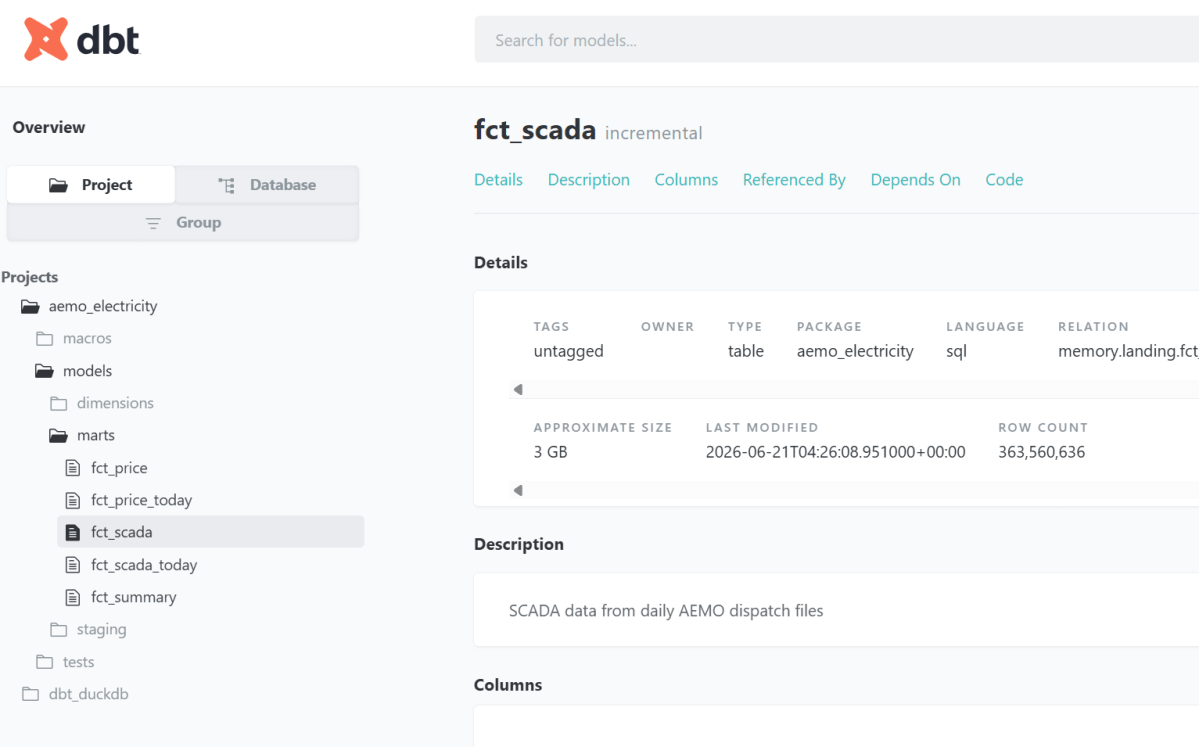
aemo, my own dbt_fabric_python_delta, built against live OneLake. The full run is published as browsable dbt docs: fct_scada is a 360M-row Delta table you can inspect yourself, not a screenshot.
snapshot_pin — a concurrent-writer test that asserts the guarantee above end to end: one writer reads a version, a second commits underneath it, and the first writer’s stale commit is rejected on real storage rather than silently overwriting.
plus a TPCH merge/append/overwrite spill benchmark, a connection-API demo on live NYC TLC taxi data, and a multi-catalog lakehouse + warehouse + local join.
The rendered catalogs for these (real Delta stats, row counts, last-modified) are on the project page.
On top of the projects, the adapter runs the official dbt adapter test suite (dbt-tests-adapter, the same conformance suite every dbt adapter is measured against) at 126/135 passing (93%), regenerated on every push to main. The documented failures are deliberate choices: no persistent views in open Delta, and rejecting merge configs that would silently diverge.
The evidence that matters is tables on real storage, hit the same way a user would, not a passing test count and not “the AI said it works.”
What does it mean to build a package you don’t understand?
I should be honest: I don’t understand the code in detail. But that was always true. duckrun is glue over DuckDB and delta-rs (written in C++ and Rust), and I don’t have the slightest idea how those work internally either. Almost nobody who builds on a library understands its guts. So what does “writing a package” actually mean?
For me, two things. Expressing the problem, knowing the pain well enough to say exactly what should happen, and making the design decisions that follow: delta-rs for every write, delta_scan views for reads, snapshot isolation as the contract. The AI writes the code; I own the problem and the shape of the solution.
The third thing is what makes it real: tests, and a lot of them. duckrun runs an extensive unit and integration suite, but I only actually trust it when I see tables land in OneLake. Code that passes locally and code that materializes correctly on real storage are not the same claim.
One trick I’ve learned: use a second agent to verify the first one’s work, not the agent that wrote it. The catch is that AI still cheats to make a test pass: it’ll weaken or game the check even when it plainly knows that isn’t the right thing. I hope that improves. Until it does: don’t trust anything it produces. Verify it against reality.
delta-rs implements the Delta Lake protocol natively. merge, update, and delete go through optimistic concurrency control on every commit. No external coordinator, no catalog service. Two writers race for the same version of the log, one wins, the other retries.
All you need is a path. No metastore to provision, no catalog endpoint, no JDBC connection, no warehouse to wake up. A folder on disk (or on ADLS / S3 / GCS) is the whole interface.
Setup: B is a Delta table being fed a series of CSV batches (batch_001.csv, batch_002.csv, …). Each merge should ingest only files B hasn’t seen yet.
A naming note: the project is delta-rs but the Python package is deltalake (pip install deltalake). On Fabric, stick with what’s preinstalled — Python notebooks already ship with deltalake and OneLake access configured.
From the notebook:
# Bootstrap target B with batch_001 already ingested
Two commits, both correct. The second run does nothing because the predicate already sees the rows. The transaction model travels with the table itself: move the folder, open it from another machine, and the next writer continues from the last commit.
write_deltalake(mode="append") and write_deltalake(mode="overwrite") are blind on purpose. Blind append means N concurrent appenders all succeed and the result is the union of their rows — exactly what you want for event streams or log ingestion. Blind overwrite means the new data wins and whatever was there is gone — what you want when the writer is the authoritative source for the table. OCC only kicks in for operations that actually read the target (merge, update, delete), since those are the only ones where a concurrent change can invalidate what you just computed.
2. I want the full read-to-write transaction, Python API is fine
A common pattern: DuckDB or Polars reads, transforms, and hands an Arrow table to delta-rs to commit. The notebook above is exactly that shape — DuckDB computes “filenames not yet in B” and delta-rs merges the result.
Inside delta-rs, OCC still works. What it cannot see is the read on the other side of the engine boundary. delta-rs knows about the merge it is about to commit; it does not know that DuckDB read B at version vB thirty seconds ago.
Carry the snapshot across the boundary by pinning both sides to the same version:
vB = DeltaTable(Target_PATH).version()
import duckdb
con = duckdb.connect()
con.sql(f"ATTACH '{Target_PATH}' AS tgt (TYPE delta, VERSION {vB});")
The OCC check now compares against vB instead of HEAD. If another process touched B in the meantime — say a parallel job deleted batch_001.csv — the pinned merge raises:
Failed to commit transaction: Commit failed: a concurrent transaction deleted data this operation read.
Catch it, recompute the diff against fresh state, retry. On the Polars side, pl.read_delta(path, version=vB) accepts the same pin, so the pattern works for any reader that exposes versioned reads.
The pin is just a number. No new infrastructure, no shared coordinator, still path-based.
3. I don’t want the Python API, I want SQL only
If you would rather write SQL — say, drive the pipeline from dbt — your options on Delta today are Spark and Fabric Data Warehouse. Both have supported dbt adapters and work great in production. I have to admit, I was hoping DuckDB would fill that gap, since it is a database and SQL-level transactions are what you expect from a database. The market went the other way: investment is going into catalog-based lakehouse formats (DuckLake, Iceberg), and the DuckDB Delta writer that does exist is tied to Unity Catalog and limited to blind appends. I don’t see them investing in a file-based conflict resolver any time soon 🙂 Lakesail seems interested in this use case, but it is still too early to call.
Takeaway
I personally use delta-rs for CSV ingestion, appends, and recording results from high-concurrency performance tests — it is fast, cheap, and bullet-proof in those scenarios. The open source maintainers are very helpful and care deeply about the product, as they use it themselves in production. But it is not the right tool for every case; Data Warehouse and Spark are more appropriate for complex workloads. With time you intuitively pick the tool that makes sense for a particular job and how much compute you can spend. None of that has to be an either/or: at the end of the day it is a lakehouse, and the whole concept of a lakehouse is having the option to choose the engine. That option matters — if we say only one engine (open source or not) is blessed for writes, then there is no point in the concept of a lakehouse.
Thanks to Frithjof for explaining Spark behaviour : The merge fixes one snapshot at transaction start (current HEAD = post-delete) and uses it for both its scan and its conflict check. Internally consistent — but bound to HEAD-at-merge-start, which Spark chose, not to the state our read saw, same behaviour when using delta_rs with a lazy dataframe : https://github.com/djouallah/Fabric_Notebooks_Demo/blob/main/TableFormat/delta/occ_spark.ipynb