All you need is Onelake

Yes, it’s clickbait. Of course you need more, but it’s hard to get anyone to read a blog these days 🙂

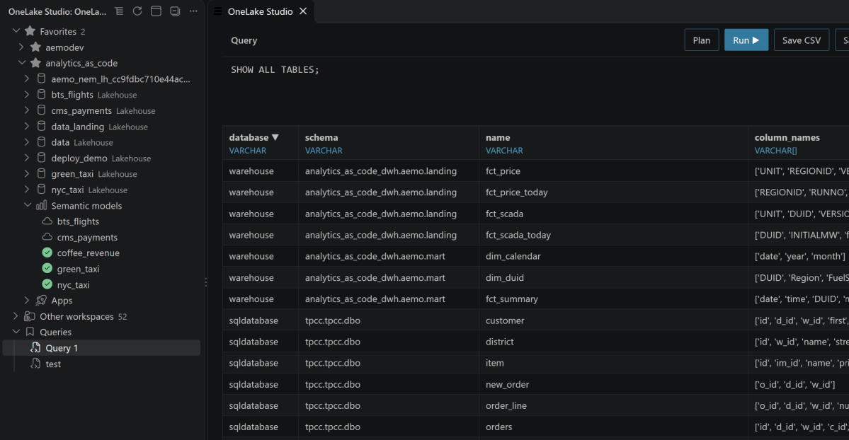
I built OneLake Studio, a free VS Code extension that treats your Fabric tenant as one catalog. Every table gets one unique name, lakehouse.workspace.item.schema.table (or warehouse.…), and every semantic model is semanticmodel.workspace.model. You explore all of it with SQL and can join across items and workspaces. It’s read only, and what you’ve opened stays cached on your machine. A semantic model (a Power BI .bim or an Apache Ossie .yaml) is a view over its tables. You can pivot it and publish it as a very basic Fabric app. The theory: if you like the app, your coding agent can turn it into a full-blown one.

Why VS Code? It handles sign-in for me (you use the account VS Code already has), and it’s where I spend all my time anyway. Authentication is still harder than it should be. I dream of a world where I never have to deal with it.

Here’s the tour: browse OneLake, look at a table, open a semantic model, explore it, see how its DAX becomes SQL, then publish it as a Fabric app your colleagues open in their browser. That last step is the point of the whole exercise. At the end is a short look under the hood.

A word of warning. This is a fun personal project, not an official Microsoft one. It computes a model’s numbers with its own engine, and matching Power BI 100% of the time is not a goal: by design it already differs, for example in case sensitivity and in how text is trimmed. The DAX compiler, dax-sql, was contributed by N.S. Devaraj.

1. Install and sign in

In VS Code, open Extensions (Ctrl+Shift+X), search for OneLake Studio and click Install. Click its icon in the activity bar, then Sign in to OneLake.

2. Browse OneLake

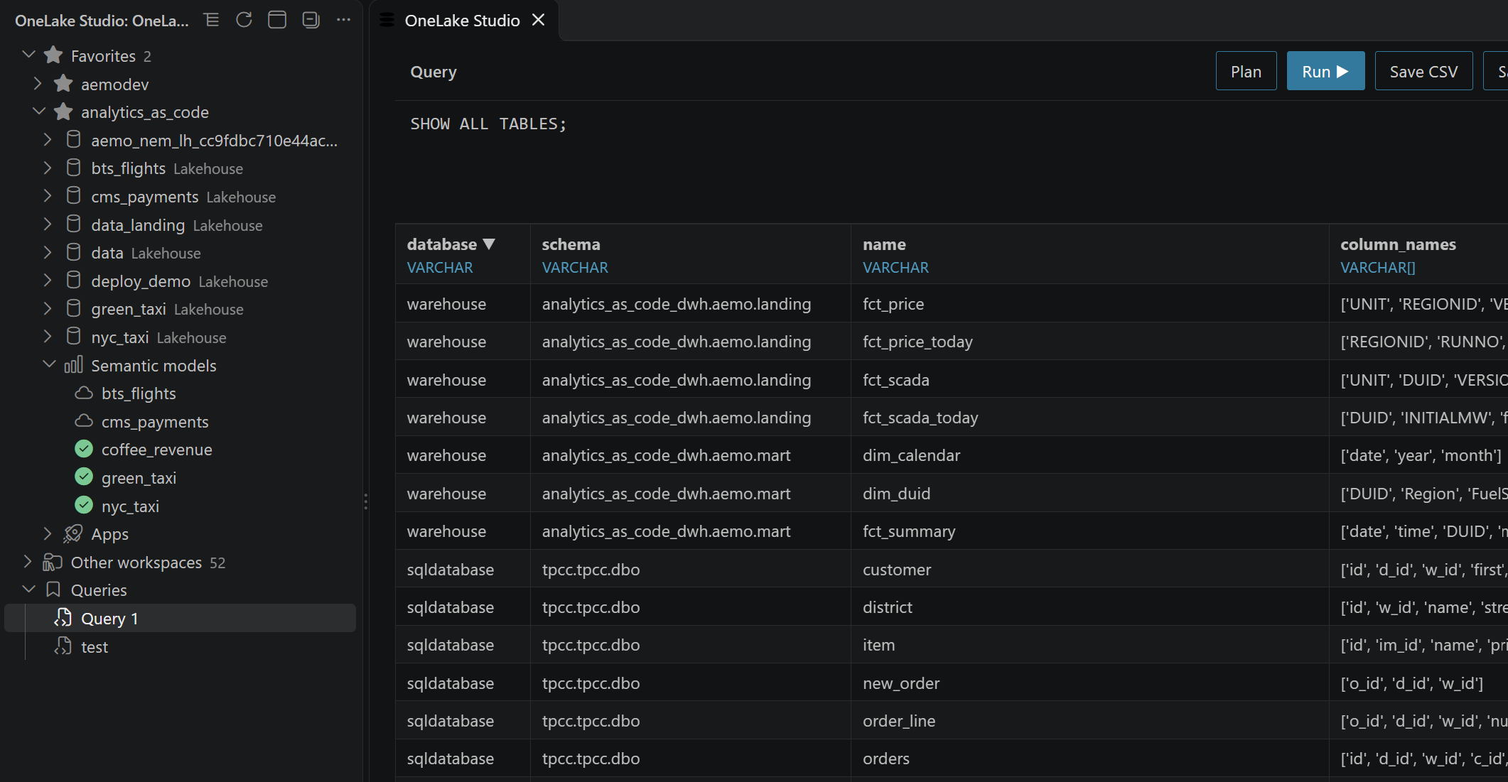
All your workspaces show up in one tree. Pin the ones you use most so they stay at the top. Each workspace lists its lakehouses, its Semantic models and its Apps. Mirrored databases show up too.
3. Look at a table

Click a table. Its icon tells you whether it was written as Delta or Iceberg, and it opens on three tabs.

Stats comes straight from the table’s metadata, before any data is read. For a Delta table, that’s its Delta log: version, rows, files, size, compression, last write, and features.
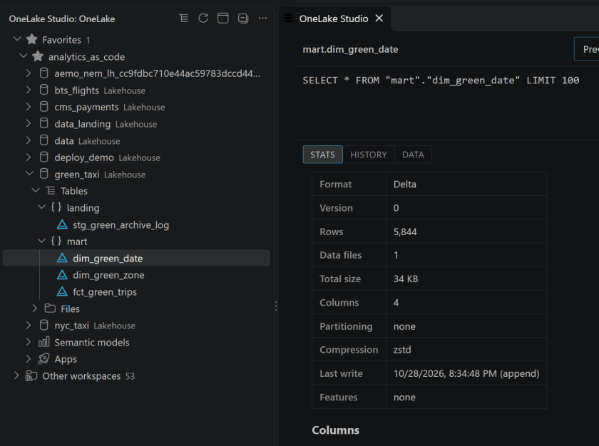
History lists what happened to the table, newest first: each commit, its operation, the rows and files it added, and which engine wrote it. Nothing is read until you open the tab.
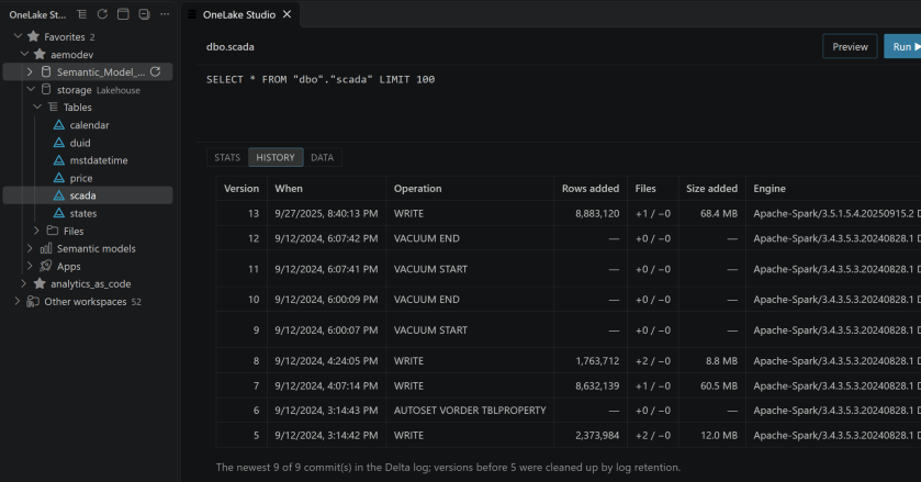
Data shows the first rows. The query is right there to edit if you want more.

Every table, Delta or Iceberg, is read through Iceberg metadata. OneLake translates Delta to Iceberg v2 by default, as a background service, and you don’t need to do anything. When a table has no Iceberg metadata, OneLake Studio quotes Fabric’s conversion log so you can see why.

4. Open a semantic model

Under Semantic models, click one. In the background, OneLake Studio saves it into its lakehouse, and a check mark shows next to it in the tree. From then on it opens at once.

The Model page shows its tables and how they relate.
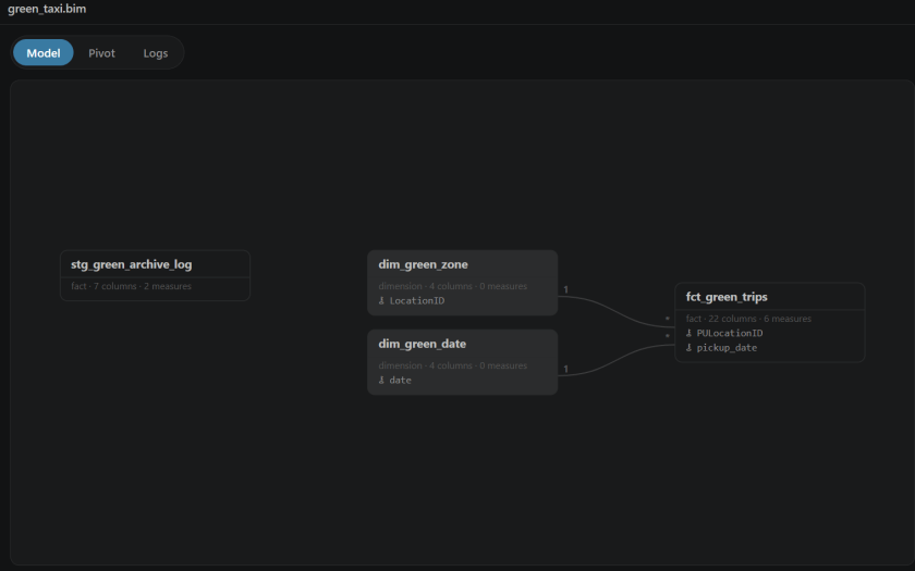
An Apache Ossie .yaml in a lakehouse’s Files opens the same way.

5. Explore it

Switch to Pivot. Drag fields onto Rows, Columns, Values and Filters, then pick a view: table, bar, line, area, heatmap and more.
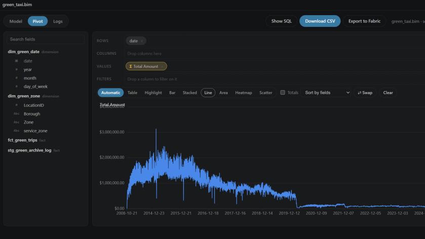
Show SQL turns the pivot into a query you can edit and run. You ask the model with plain SQL. Pick your columns, wrap a measure in AGG(), and select FROM model. For example, on the NYC taxi model:

SELECT "dim_date"."year", "dim_zone"."Borough", AGG("Total Amount")
FROM model
GROUP BY ALL

AGG("Total Amount") is the measure exactly as it was defined in the model, in DAX. It’s computed in the context of each row (that year and that borough, plus any WHERE you add), just like a visual in Power BI. There’s no new syntax to change a measure on the fly, to add a filter or remove one, and I’m not interested in inventing one. If you need a different calculation, define it in the model.

Show SQL also shows where the time went.
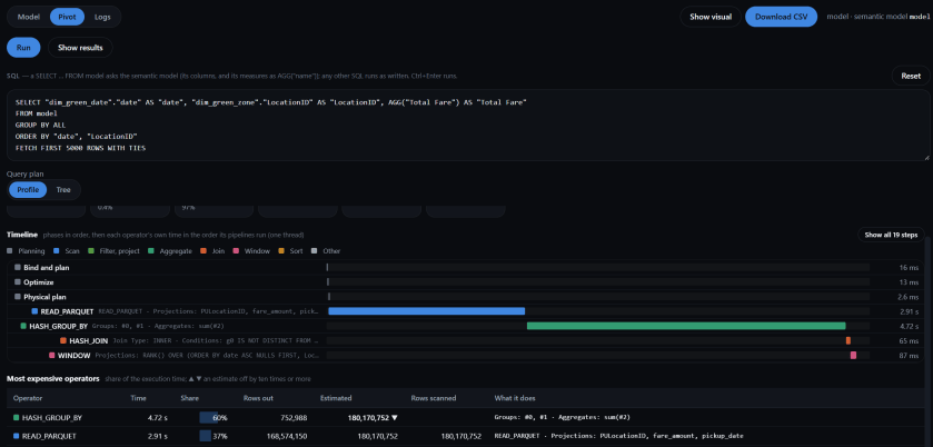
Click Tree to see what actually ran. You never wrote a join, but the model knows how its tables relate, so the trips are joined to the zones on the location and to the calendar on the date. Only the columns the query needs are read.
6. DAX to SQL

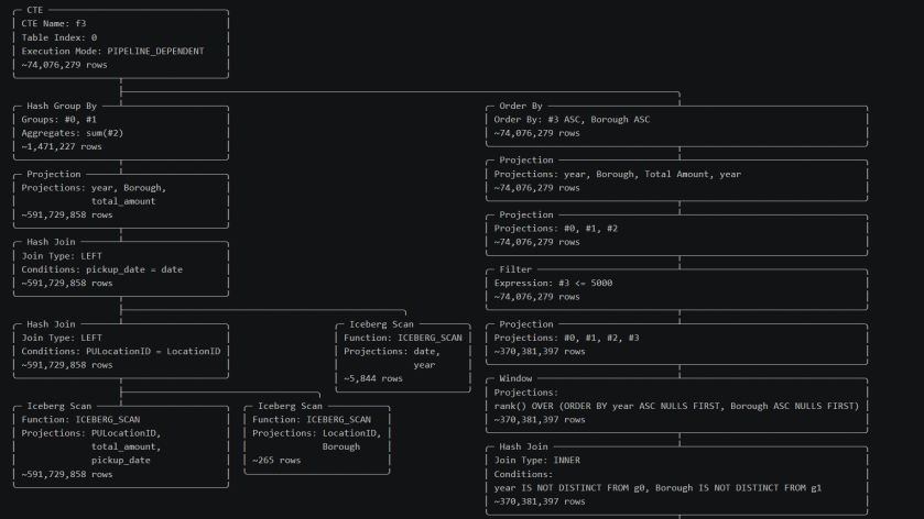
Every measure goes through dax-sql, a compiler that turns DAX into plain SQL, which DuckDB then runs. Here it is on something less trivial than a SUM: each borough’s share of the year’s total.

DEFINE MEASURE fct_trips[Share of Borough] =
DIVIDE([Total Amount], CALCULATE([Total Amount], ALL(dim_zone[Borough])))
EVALUATE SUMMARIZECOLUMNS(dim_date[year], dim_zone[Borough], "Share", [Share of Borough])

That compiles to this (only the line breaks are mine):

WITH f3 AS MATERIALIZED (
SELECT j4."year" AS "g0", j5."Borough" AS "g1", SUM(t2."total_amount") AS "a0"
FROM "mart"."fct_trips" AS t2
LEFT JOIN "mart"."dim_date" AS j4 ON j4."date" = t2."pickup_date"
LEFT JOIN "mart"."dim_zone" AS j5 ON j5."LocationID" = t2."PULocationID"
GROUP BY j4."year", j5."Borough"),
f7 AS (SELECT f3.g0 AS g0, SUM(f3.a0) AS a0 FROM f3 GROUP BY f3.g0)
SELECT CAST(q10."year" AS BIGINT) AS "year", q10."Borough" AS "Borough",
CAST(q10."Share" AS DOUBLE) AS "Share"
FROM (SELECT s9."year", s9."Borough", s9."Share"
FROM (SELECT *
FROM (SELECT k1."year" AS "year", k1."Borough" AS "Borough",
(f3.a0 / NULLIF(f7.a0, 0)) AS "Share"
FROM (SELECT f3.g0 AS "year", f3.g1 AS "Borough" FROM f3) AS k1
LEFT JOIN f3 ON f3.g0 IS NOT DISTINCT FROM k1."year"
AND f3.g1 IS NOT DISTINCT FROM k1."Borough"
LEFT JOIN f7 ON f7.g0 IS NOT DISTINCT FROM k1."year") AS z8
WHERE z8."Share" IS NOT NULL) AS s9) AS q10

A few things to notice:

  • ALL(dim_zone[Borough]) doesn’t scan the trips again. f3 is the total by year and borough, and f7 adds the boroughs up for each year. The fact table is read once.
  • DIVIDE divides by NULLIF(…, 0), so a zero total gives a blank, not an error.
  • Blank rows are dropped, as SUMMARIZECOLUMNS does.

7. Publish it as a Fabric app

Click Export to Fabric. Confirm where the local copy goes and click Export.
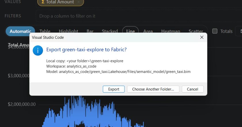
Once it’s published, your colleagues get the same pages in their browser, without VS Code.
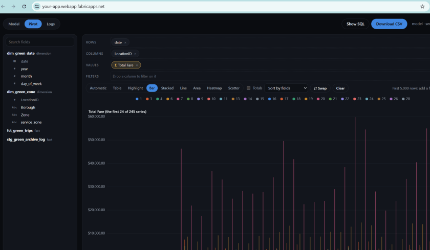
The app lives in your workspace, protected like any other Fabric item, so only people with access can open it (it shows under Apps in the tree, with a lock). It reads the model where it lives, so nothing is copied and the data is current. And a copy of the app stays in your folder, so you can treat it as a starting point: change it, then export again.

How it works

The same pages (Model, Pivot, Logs) run in two places, on DuckDB both times.

  • In VS Code, the extension runs a native DuckDB 2.0 inside VS Code itself. It’s multithreaded and reads OneLake directly, with the token from your VS Code sign-in. The panel you see is only a view.
  • In the Fabric app, there’s no VS Code, so the engine is DuckDB-WASM 1.5.6, running in the viewer’s browser. The app is a static page plus one small function. The function runs in Fabric: it reads the model from the lakehouse and tells the page where each table is. The page downloads the Parquet files it needs, and DuckDB reads them from the browser’s local storage. SQL typed in the app only sees those Parquet files and can’t read anything else.
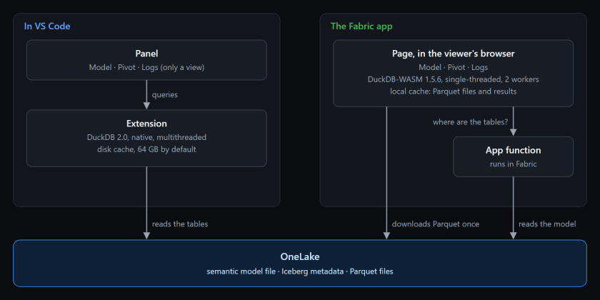
DuckDB in the browser: single-threaded

DuckDB-WASM runs single-threaded here, so one query always runs on one core. A big scan is noticeably slower than the same query in VS Code. To keep the page responsive, the app runs a pool of two engines, each in its own web worker, fed by one queue. When a page draws several visuals, two queries run side by side, and a slow one holds up only its own engine. (I tried three. It wasn’t faster.)

I also tried a multithreaded build. It turned out to be more complex than it looks, so for now it stays single-threaded, and the pool of two does the job.

The cache

Iceberg files never change once they’re written, so almost everything can be kept.

  • In VS Code, listings, table metadata and first rows are kept on disk. They’re shown at once and refreshed in the background. Table data goes into DuckDB’s disk cache (64 GB by default, per account), so a table you’ve read before comes from your machine, even after a restart. Clear Cached OneLake Data empties it.
  • In the browser, there are four layers:
    • The function’s answer (where the tables are), kept for about an hour. A viewer calls the function about once an hour, not on every load.
    • The Iceberg manifests, so a new snapshot reads only the manifests it added.
    • The Parquet files, in the browser’s private file system (OPFS), up to 64 GB, shared by both engines and every tab. This is why the app needs Chrome or Edge 121 or later.
    • Query results, stored as Arrow and keyed by the SQL and the tables’ current snapshot. A reload answers every query it has already seen without running the engine. New data means a new key, so you never see a stale result.

Each app has its own cache, in each browser. The first visit pays for the download. Later visits are fast.

Limitations, by design

Everything runs on the client: the engine on your machine (or in your colleague’s browser, for the Fabric app) reads the data straight from OneLake.

  • Egress fees can become a problem. Every query pulls data out of OneLake to wherever the client is, and with big tables or users far from the data, that can cost money.
  • Row- and column-level security (RLS/CLS) aren’t supported. OneLake now has a table read API (in preview) that returns Apache Arrow with RLS and CLS applied. I’ve tested it with Python and it works as expected, but I haven’t tried it with WebAssembly yet.
  • It’s for small data. Don’t use it to download 10 GB tables.
  • Correct SQL is not the same as a good plan. Even when the generated SQL is right in theory, getting a well-optimized plan out of it is not obvious at all. A measure becomes CTEs, re-aggregations and joins that nobody would write by hand, and the engine has to see through them. Some queries will be slower than they should be.
  • DAX to SQL comes with no guarantee. dax-sql, contributed by N.S. Devaraj, compiles DAX as faithfully as it can, but there’s no guarantee that a result is correct, or that a given function or piece of syntax is supported. Some DAX isn’t supported at all.

So it’s not meant for production or any serious setup. But it’s an interesting experiment in what a Fabric app can do on its own, IMHO.

Funny enough, I wrote about this back in 2021: BI tools need a SQL generator that composes measures the way Power BI does, including the ones that ignore your filters. I had the idea, but obviously I couldn’t build it. Five years later, with AI, I could. If anything, this project is a testament to how far AI has come.

Try it

Install OneLake Studio from the VS Code Marketplace. It runs on Windows, macOS and Linux.
Iceberg on a single node is coming together

For a long time, whenever I tried to use Iceberg outside the JVM ecosystem, something I needed seemed to be waiting for the next release. It took longer than I hoped, but lately I have been able to get much further with the engines I use.

chDB can authenticate to OneLake with a token, Polars now runs all 22 queries in this benchmark, and DuckDB’s cache feels like absolute magic on the second pass. I still ran into bugs, but I could run both reads and writes across several engines against the same Iceberg catalog.

I took two of my notebooks and port them to GitHub Actions as python script across DuckDB, Polars, chDB, LakeSail, Spark and Daft. One runs analytical queries; the other reads CSVs and writes Iceberg tables. I wanted to see how each handled the workloads on a small 4-core runner.

The data lives in OneLake. Reading through its Iceberg REST catalog is already available; the write support I used is still in private preview.

Both benchmarks run on a public 4 vCPU / 16 GB runner. The engines connect to the catalog either directly or through pyiceberg. OIDC federation provides a token per job, so there is no client secret to store. The same approach should work with other Iceberg REST catalogs, provided the engine supports their storage and authentication.

The code, the raw JSON of every run and the charts are in djouallah/lakehouse_benchmark.

Reading: TPC-H-like queries at SF10

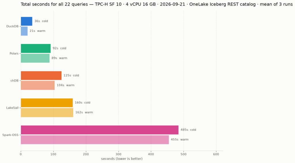
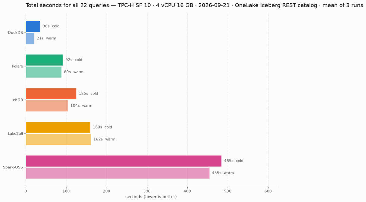
The tables are generated with tpchgen, uploaded as Parquet and registered with pyiceberg’s add_files. DuckDB and LakeSail could have written them just fine, but I wanted to stay neutral. Each engine attaches the catalog, runs the 22 queries, then runs the same 22 again immediately. Those are the cold and warm passes below; catalog attach time is excluded. The chart and the table are the mean of three runs on 20 and 21 September 2026. This is a small single-node comparison, not an official TPC-H benchmark.

EngineVersionColdWarm
DuckDB2.0.0 dev35.9s21.3s
Polars2.0.0-rc.292.1s88.6s
chDB4.4.0125.4s104.5s
LakeSail0.7.1159.9s161.6s
Spark-OSS4.1.3484.9s454.9s

Spark open source, not to be confused with Fabric Spark, is a single-node JVM on 4 cores here. Thanks to AI, running Spark locally is no longer a scary experience. Unfortunately Daft is missing: at 0.7.25 it runs 16 of the 22 queries, because l_extendedprice * (1 - l_discount) overflows its decimal precision ceiling of 38 (Daft#7532). I like Daft and would love to include it in the full query comparison once this is fixed. It does complete the ETL workload below.

Writing: Light ETL

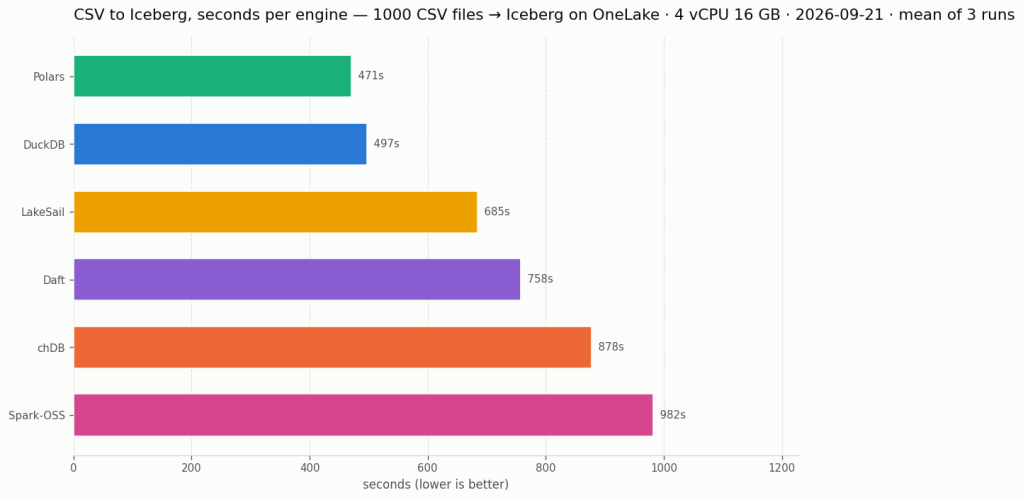
1000 daily AEMO CSV files, 52 GB, are landed once in the lakehouse Files/ section. Each engine reads all of them, filters, casts and writes one Iceberg table of 149,146,763 rows through the same catalog. DuckDB, LakeSail and Spark have their own Iceberg writer. chDB and Polars stream Arrow batches into pyiceberg. Daft has its own writer over a pyiceberg table.

EngineLoad
Polars470.8s
DuckDB497.4s
LakeSail684.5s
Daft757.9s
chDB878.1s
Spark-OSS982.2s

Every engine ends with the same row count. Load time includes recreating the table, reading the CSVs, transforming, writing and committing; session setup and catalog attach are timed separately. There is one load pass per engine, and the chart and the table are the mean of three runs. Snapshot isolation and concurrent writes will have to wait for another blog. The Iceberg write path used here is in private preview.

Random learnings, in no particular order

  • DuckDB needed AZURE_TRANSPORT_OPTION_TYPE=curl on this Linux runner. Without it the Iceberg attach succeeds and every data-file read fails with a message that looks exactly like a missing credential. Setting the transport fixed it. I had not seen this in the Fabric notebook.
  • chDB returned 41 rows for Q13, everybody else 42. ClickHouse defaults join_use_nulls=0 and fills unmatched outer-join cells with default values instead of NULL. The row-count smoke test caught this, and the benchmark now sets join_use_nulls=1.
  • The catalog cache settings do not all mean the same thing. I configured a 15-minute lifetime, but LakeSail’s “table cache” caches the table listing, not the loaded table. It still loads table metadata on every statement, adding REST requests even on the warm pass (sail#2629).
  • Daft’s six query failures come from decimal arithmetic. CTEs, EXISTS and correlated subqueries all work. It also rejects backticks outright, which looked like a total dialect failure until I read the error. Separately, its Azure URI parser drops the container on OneLake hosts; the bench works around it with az:// paths. The proposed fix is Daft#7533.
  • Nothing is partitioned, on purpose. The pyiceberg streaming append used here only supports unpartitioned tables. A first version that materialised batches to partition by year took the 16 GB runner down at 100 files. So every engine writes the same unpartitioned shape and year stays a plain column.

Spark, and why it has no native accelerator here

Spark-OSS is 4.1.3 with Iceberg 1.11 and hadoop-azure 3.4.2. I also looked at Comet and Gluten/Velox, but could not use either for this benchmark.

  • Comet supports Spark 4.1 and ships a native Iceberg reader, but its readable schemes are file, s3, s3a, gs, oss. An abfss table is declined at planning time and runs on the JVM as if the plugin were not there. I left Comet out because it could not accelerate these scans. Filed as datafusion-comet#6058.
  • Gluten/Velox has a Velox ABFS connector, but I could not find a published package for Spark 4.x to test (This basically what Fabric NEE uses)

Conclusion

All six engines completed the CSV-to-Iceberg load. Five completed all 22 read queries; Daft completed 16. Being able to try this many engines against one catalog, with the data staying in OneLake, is what I find exciting. chDB’s token support and Polars running all 22 SQL queries give me more options for the notebooks I already use.

DuckDB was fastest on the reads, and on the load it traded first place with Polars from run to run. DuckDB’s read total fell from 36s to 21s on the second pass, about 40%. The other engines improved less, and LakeSail’s warm pass came out slightly slower than its cold one. That makes repeated reads worth testing separately from a one-pass load. It does not tell us exactly what each engine cached or how many bytes it fetched; chDB also has a filesystem cache configured here.

For my ETL workload, the cache does not matter: read the new files, transform them and write the table.

If you want to see how much things have changed, have a look at these TPC-H SF10 results from four years ago.

Note: The write benchmark requires access to the private preview used here coming soon.

Writing Databricks Parquet That VertiPaq Likes

This post, the repo and every number in it are personal opinion. Nothing here is a Fabric position, benchmark or recommendation.

My colleague Eiki published a post on Microsoft’s white paper on Power BI architecture choices for Azure Databricks. Read it first: it covers the four storage modes, the headline findings, and links to the paper. I assume you know what the paper measured.

I like the paper for a different reason. It benchmarks a lakehouse as designed: open files on object storage, one vendor writes, another reads, Parquet is the only contract. Such benchmarks are rare, hard to reproduce and usually opinionated. This one is deliberately neutral (maybe too neutral) , The dataset is so uniform that V-Order has little room to differentiate the writers, so all writers start on relatively equal ground.

I have written before about VertiPaq reading Parquet that other engines wrote: Optimizing Parquet Layout for Power BI Direct Lake Mode (Dec 2024), Just VOrder, don’t try to understand how VertiPaq works (Nov 2025) and Writing Parquet That VertiPaq Likes (Aug 2026).

The short version: VertiPaq reads Parquet from any producer. It does not need V-Order. It prefers a layout it can transcode fast and hold small, and V-Order is one way to produce it.

This post applies that idea to Spark on Databricks. I am not a Spark expert; I know delta-rs much better. The Parquet concepts carry over, the knobs do not, and Databricks has many settings that interact.

AI helped me navigate them. Where the repo gets Spark wrong, the mistake is mine. Corrections welcome.

What I did

The paper tunes the Databricks write with the mainstream, documented settings, as an industry paper has to. This is a personal blog, so I can be less orthodox and go low level 🙂 I tried a few little-known knobs instead.

All of them are cluster configuration for row-group size and dictionary encoding, the same lines for every table, plus one optional step per fact table: a single clustering key on the column the reports filter on (nothing fancy it is just a global sort).

I used the paper’s protocol: TPC-DS at SF100 and SF1000, its DAX capture, 20 concurrent readers, three load tests back to back on one model. Two changes: the semantic model is deleted after the three runs so the next run starts cold, and the OneLake cache is on because my Databricks tenant is in another region. Only the very first run at a scale factor reads across regions; every later run 1 reads from the cache, so it measures the transcode alone.

Note: I used Fabric layout as it is.

Databricks writes, Direct Lake reads through the mirrored catalog. The configuration, what each line does and what breaks it are in the repo. This post is results only.

The results

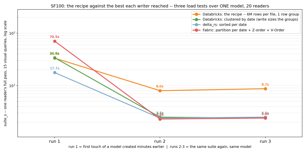
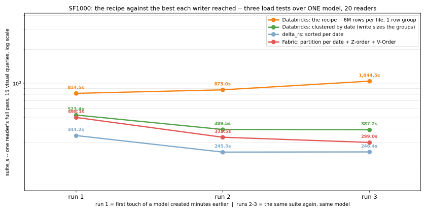
Each chart shows the configuration alone, the configuration with the clustering key, and the best layout of each other writer: delta-rs sorted on the date key, and the paper’s Fabric layout of one partition per date with Z-order and V-Order.

Run 1 pays the transcode; runs 2 and 3 rerun the same queries on the loaded model.

At SF100, the configuration alone produces dictionary encoding and large row groups, but is about three times slower than every ordered layout. Adding the clustering key on the date matches the paper’s V-Order layout, with row groups more than ten times larger.

At SF1000, the configuration alone never really warms up: each run is slower than the last, while the three ordered layouts do. That is why the clustering key is not just an optimisation in the recipe; it is what makes the layout usable at this scale. The clustered arm still trails delta-rs and the paper’s layout at SF1000: the clustering did not fully sort the rows at that scale, and the repo carries that as open. Why delta-rs has the best cold run at both scale factors is still a mystery to me.

The interesting part is that VertiPaq does not care who wrote the Parquet. It cares about the physical layout it has to transcode.

The repo

github.com/djouallah/parquet_layout_vertipaq_spark has the configuration, the clustering step, what undoes it, the numbers behind both charts and what is still open.

It also ships a Claude Code skill that applies the recipe.

AI, dbt and Iceberg are already changing data engineering

I have been using AI in VS Code and Onelake, initially trying to make sense of Chat with your data (without much success, that thing is very hard and we need some breakthrough), and more recently for data engineering. I noticed something: AI has become useful enough in the last couple of months that it is changing my workflow.

None of the individual pieces here is new or particularly interesting by itself. But combine them and we have something!!! CI/CD, Iceberg REST catalog, Opus 4.8, me discovering how OIDC GitHub integration works in Fabric, and dbt, and suddenly everything makes more sense.

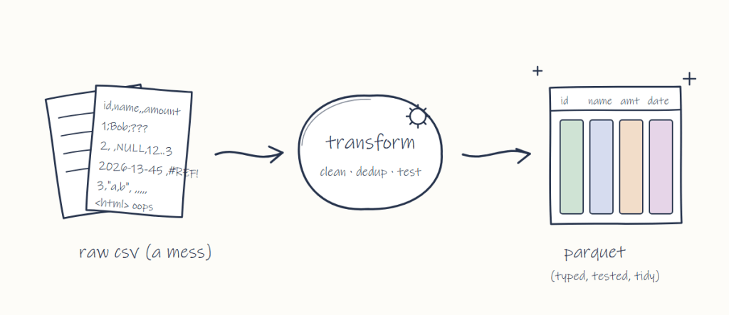
Let’s take a simple ETL job, read some CSV, clean it, and produce high quality Parquet files that humans and AI can consume.

From a human perspective, and although we like to think our judgement is based purely on cost and performance, that’s never really been the case. It is always influenced by personal bias: Spark people will always use Spark, T-SQL people will always use the DWH, and Pandas people don’t care, they will use their thing.

Now, if we imagine an AI doing that, the incentives are different. Yes, AI is biased by its training data, but it isn’t biased by tribe. Judging by my AI agent (I suspect it is telling me what I want to hear), it doesn’t care. It prefers short loops, and if you tell it “I want the cheapest option”, it is smart enough to try to do that.

1- ETL is just processing raw data into something coherent that can be consumed. It is a deterministic process, and as someone who mainly used GUI tools, it took me a while to get it: data engineering is just code!!! Those tools are writing code, it just happens that we don’t see it 🙂

2- All things considered, an AI agent has no personal attachment to an engine, assuming you give it a strict spec. An agent will not favour an engine because of familiarity, or because it spent so much time using it that it became tribal.

3- Opus 4.8 class AI is good enough for general purpose data engineering. The current issue is the cost. Right now you need a Max subscription in practise and it is just not sustainable, but I am confident the market will figure out a solution. We don’t need AGI, just a super cheap Opus 5 alternative 🙂

4- I am not saying all engines are equal, or that they become just a SQL runtime. That’s not true. But because the cost of switching from one SQL dialect to another is minimal, the human excuse of “I use what I know” (which is pretty tragic, when you think about it) will no longer be relevant.

Selecting an engine will be strictly based on facts: engine 1 can do efficient MERGE, engine 2 cannot, engine 1 wins. That’s fair.

And engines still have a lot to improve, see for example non-trivial incremental processing, async remote scans, partial caching, Dynamic Horizontal scaling etc.

And to be fair, the dialect alone is not the whole story. Subtle differences in engine behaviour, even when using the same SQL text, can be a pain. I learnt this the hard way. I spent too much time trying to debug a result, only to find out that two engines have different behaviour when doing a join using a word with padding: “spain” and “spain ” may or may not mean the same thing.

But the good thing is that a cross-engine parity check catches these subtleties automatically. Either the numbers match or they don’t (you can’t do that with Chat with your data).

5- Cloud storage vendors ultimately want to store more data, regardless of how it was processed — their incentives are aligned with this agentic trend. In my personal opinion, they need to spend less time on MCP and other AI stuff, and just focus on the boring stuff: authentication, documentation, and interoperability.

If you want to deviate from the catalog spec, at least spend some engineering time working with the open source engines to support your own variant.

6- The less a client has to do, the better for everyone: move more stuff to the catalog, including table scanning and server-side planning.

A read-only client has no interest in reading Avro files. Just give me a list of Parquet files and deletion vectors to read. Keep it opaque. Store it in a database, I don’t care. Just give me the data files to read.

7-I added this note because of early feedback on the blog, which was basically: “I don’t care about Iceberg, I use Delta.” That’s a fair reaction. The good news is it won’t really matter — Delta 5 will use the same adaptive metadata as Iceberg V4. They’re still two separate projects with different governance model(or rather, the lack of it), but ultimately they’ll produce the same thing in theory . Just give it another 2 years or so, there is a real table format fatigure, translating from one to another is a waste of everyone time, and to be honest, some vendors find it is much cheaper just to lock users using credential vending instead of weaponising the table format 🙂

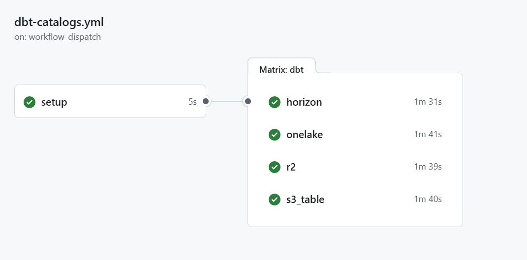
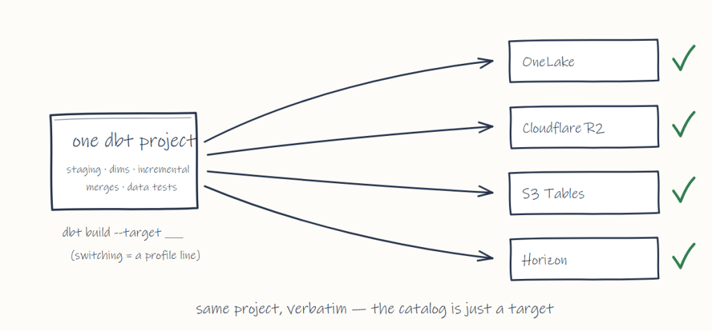
Instead of another abstract “thought leadership” blog post 🙂 here’s a concrete example: the same dbt project, unchanged, runs against four different vendors’ Iceberg REST catalogs: OneLake, Cloudflare R2, S3 Tables and Snowflake Horizon, each in about a minute, on a throwaway GitHub Actions runner with DuckDB as the engine.

Switching catalog is literally changing one ATTACH in profiles.yml.

The whole thing is public: testing-iceberg-rest-catalog.

Hopefully, data engineering will move away from configuring and fine-tuning engines and towards talking more to end users and understanding what they need: agreeing on what the numbers are supposed to mean, and writing the tests that catch it when they are wrong.

The machine can build the pipeline, and it will probably be better than us at it, but it doesn’t know what “correct” means. I was tempted to write something about ontology but I am not going there 🙂

And getting access to that ERP will always require a human. That’s an organizational thing, and no AI can fix it.

As a data analyst by trade, I always found data engineering a chore. I never enjoyed it , and to be honest ,it does not bother me if writing transformation becomes fully automated

So I have a bias, to be honest, and maybe this blog is just wishful thinking. But what if it is true? I think, at least, pay attention to this new trend.