Writing Parquet That VertiPaq Likes

This rabbit hole started with a simple observation: VertiPaq seemed to like parquet produced by delta-rs more than parquet produced by DuckDB — and that drove me nuts. delta-rs was at the time a niche library for nerds; Fabric didn’t even have a Python notebook. The mental model was simple: write with Spark, get V-Order, get the best possible layout for Power BI.

It is 2026; Fabric is more widespread, and there are simply more patterns and use cases:

  • New Fabric workspaces default Spark to the writeHeavy resource profile, which does not write V-Order.
  • Customers — especially on smaller SKUs — routinely write with delta-rs from Python notebooks.
  • Reading tables written by Snowflake, Databricks and BigQuery through Direct Lake is a production pattern.

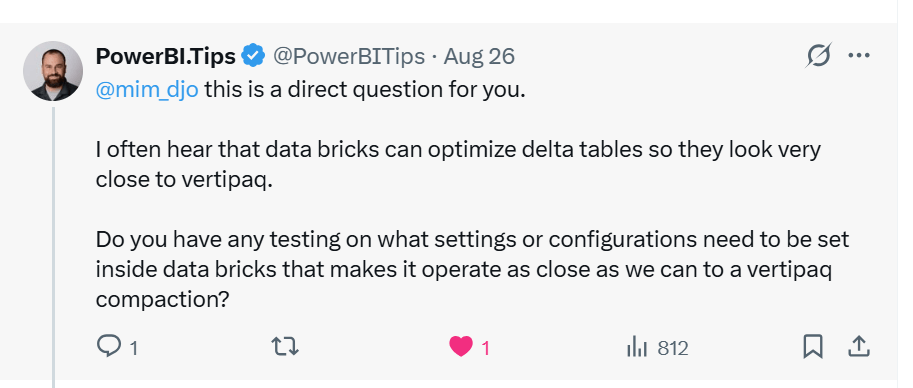
So “what parquet is friendly to Vertipaq” is now a legitimate data engineering question — I can’t tell you how happy I was when I read this tweet 🙂
The short version

  1. Row groups of a few million rows : 2–6M rows per group; never go above 16M, VertiPaq’s segment ceiling.
  2. Dictionary-encode every column — and make the file footer say so.
  3. One global ORDER BY, lowest-cardinality columns first, date up front. No clustering, no Z-ordering, none of that.
  4. Delta vs Iceberg does not matter. Only the parquet inside the table matters.

Method

I treated VertiPaq as a black box and did what experimental science does with a phenomenon it doesn’t understand: change one variable, measure, repeat. Nothing here is confidential or internal — every number was measured from the outside, on tables anyone can rebuild.

One more thing changed this year: AI became genuinely useful for this kind of work, because it never gets bored. Sweeping writers × row-group sizes × file sizes × sort orders across hundreds of runs is exactly the tedium it doesn’t feel.

Two experiments.

  • First: figure out why VertiPaq preferred delta-rs output.
  • Second: run multiple writers and vary row-group count, file size and ordering, measuring cold, warm and hot query cost.

Caveat. Hot behaviour is well documented — after all, it is the same in-memory format as import mode — so I am more interested in cold runs (first touch of a fresh model), even though most real-world traffic is hot: a live model transcodes once and then serves from RAM.

The datasets are rather smallish — the biggest table here is around 600M rows. As a data analyst I have always dealt with small data, so I am optimising for the workload I actually care about.

How Direct Lake reads your parquet

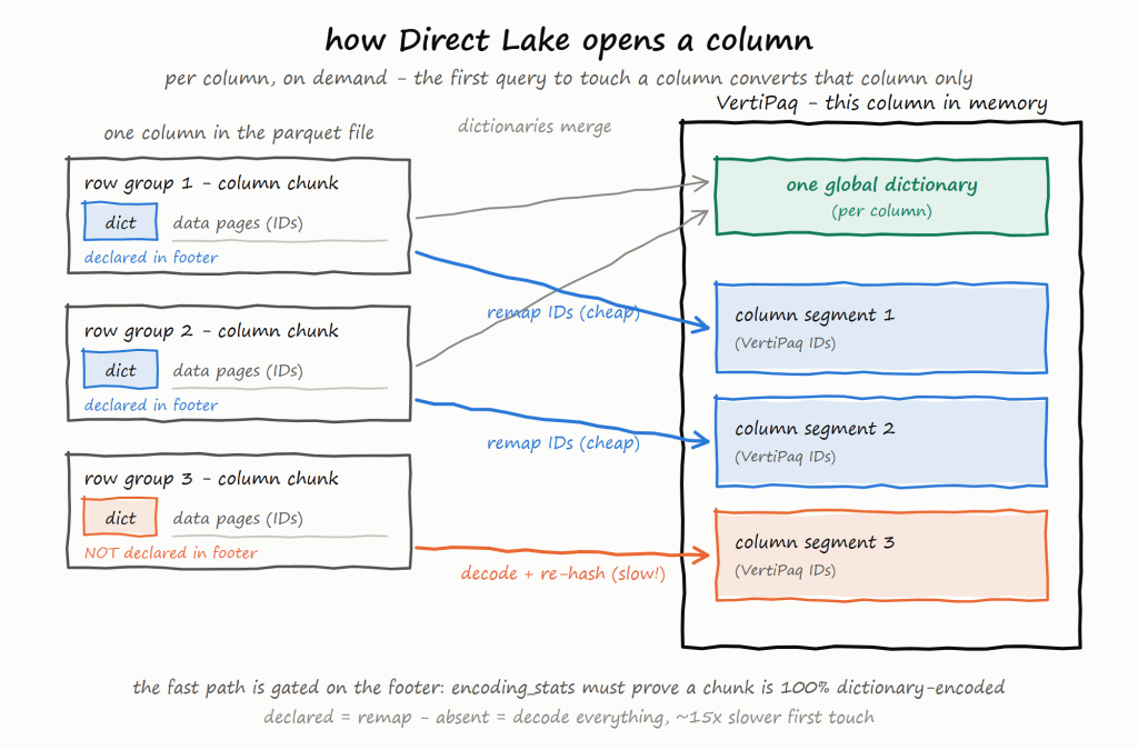
The mechanism that explains almost every finding. Transcoding is per column, on demand: the first DAX query to touch a column that is not yet in memory converts that column only into VertiPaq’s in-memory format. The column’s per-row-group parquet dictionaries are merged into one global VertiPaq dictionary, and each row group of the column is loaded as one resident column segment, remapping parquet data IDs onto VertiPaq IDs on the way in. Every query after that scans the segments the transcode produced. Query latency — and capacity consumption — is therefore a property of how the parquet was written.
Findings

Dictionary encoding is the big one

VertiPaq is itself a dictionary-based engine. When a chunk arrives dictionary-encoded, the transcode merges the parquet dictionary into the column’s global one and remaps the data IDs — it never decodes the values. Anything else has to be decoded and re-hashed, value by value, at load time. On a single 144M-row DECIMAL(18,4) column, PLAIN measured 618.6 MB against 423.1 MB dictionary-encoded — ~200 MB extra and a re-encode, on one column.

The surprise is that the encoding alone isn’t enough: the declaration is part of the encoding. The engine takes the cheap remap path only when the footer’s encoding_stats prove a chunk is entirely dictionary-encoded without decoding its pages. DuckDB’s writer emitted no encoding_stats at all until duckdb#24957 (merged 2026-08-24, currently in main only). That PR measures the cold first-touch of a 142M-row dictionary string column falling from 10,857.5 ms to 689.3 ms — about 15×, with identical pages. The attribution was verified the hard way: synthesising only that footer field into an otherwise unmodified file reproduces the speedup. A second PR, duckdb#24645 (merged 2026-08-10), adds a data_page_size_limit option — before it, DuckDB often wrote one huge data page per column chunk.

Row-group size: a tension between cold and hot

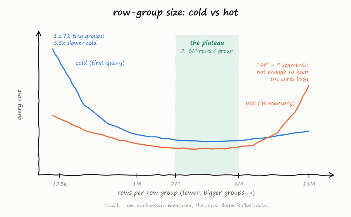
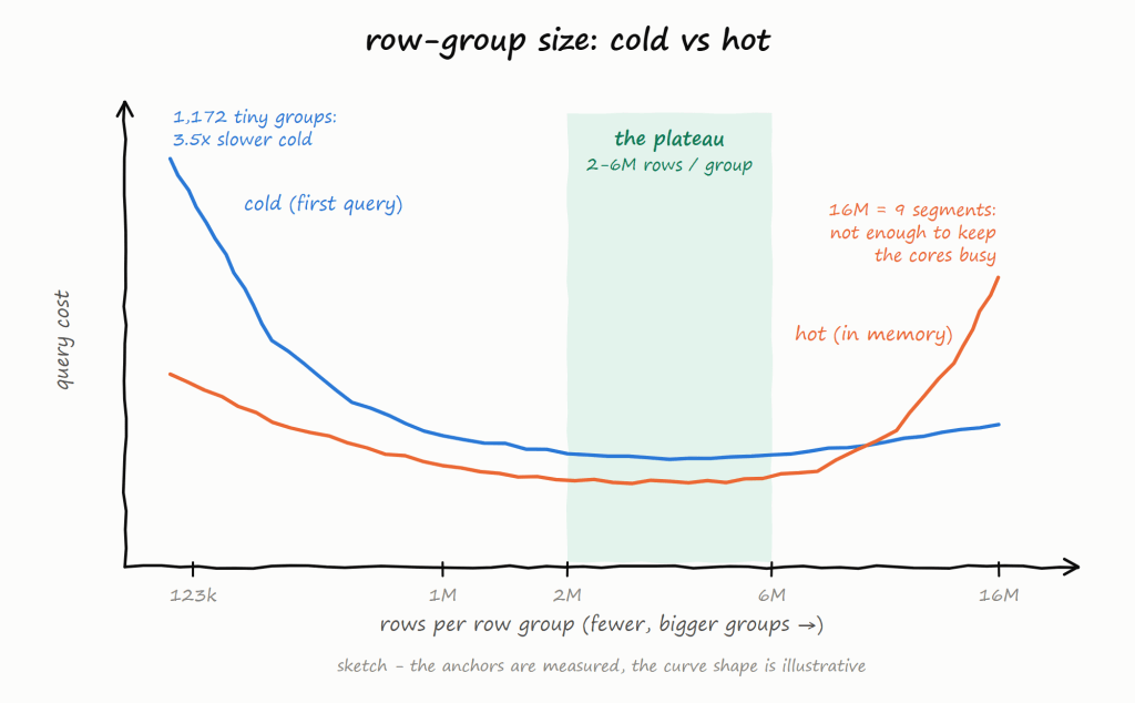
There is no single best size, but both ends fail measurably. Every row group is one more dictionary merge and one more segment to set up per column, which is why tiny groups murder the cold tier: the same DuckDB in the same notebook was 3.5× slower cold (96,503 ms vs 27,785 ms) when a library default sliced a 144M-row table into 1,172 groups of ~123k rows. At the other end, 16M rows — VertiPaq’s segment ceiling — was the worst sorted geometry measured: nine segments starve the scan pool. Cold prefers slightly bigger groups than hot, but very big groups are bad for both.

Power BI doesn’t disclose how many cores it uses, so the practical rule is: enough row groups to keep the cores busy. On the 144M-row table, warm query time stepped down between 19 and 24 groups (≈5,700 ms → 3,221 ms), and 72 groups bought nothing over 24. Hence the plateau: 2–6M rows per group.
A global sort keeps paying after the data is in memory

Transcoding does not change row order — it is essentially a working data copy into memory. So a sort applied at write time survives into the resident segments, which is why ordering matters for hot runs too, not just for compression.

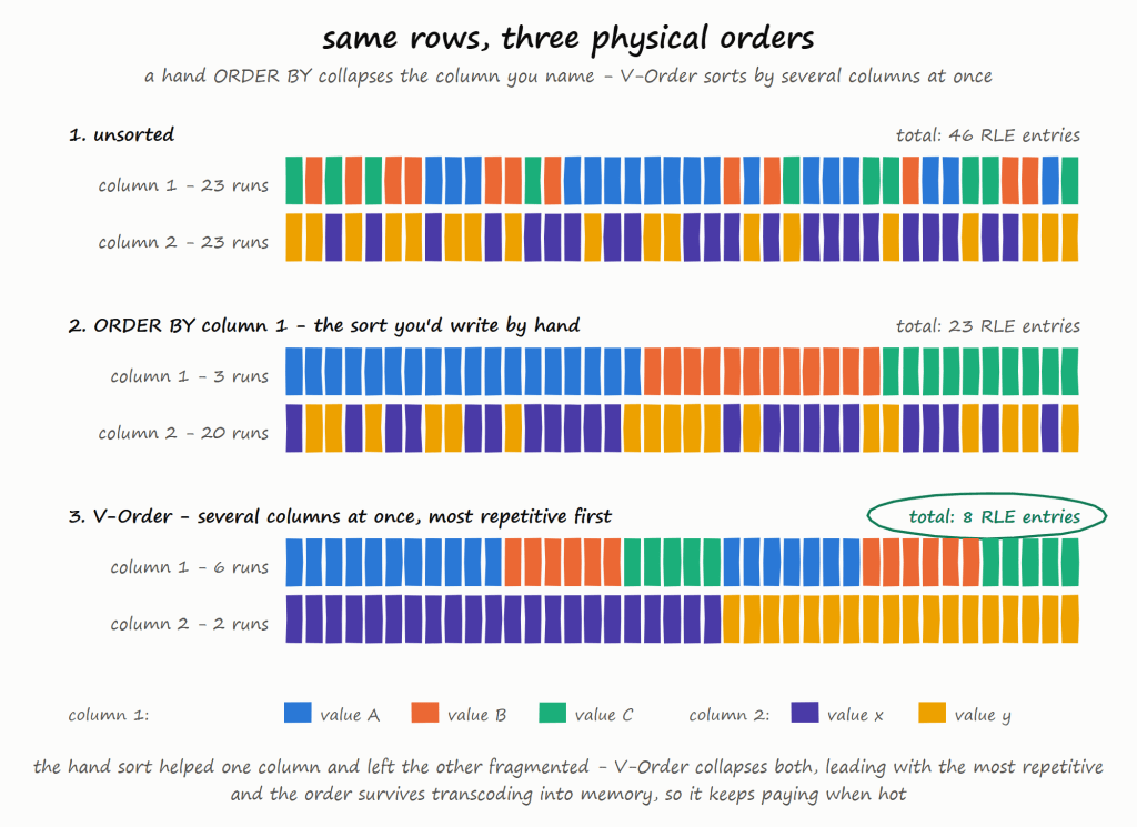
A single global ORDER BY with low-cardinality columns first (and a preference for date) produces long RLE runs. It is not V-Order — but in some cases it is good enough. When V-Order does engage, what it’s worth depends on the surface — column count × categorical skew — not row count: on a skewed 17-column taxi table it collapsed the most repetitive column to 3,371× fewer runs; on a near-unique 5-column table it left row order untouched and still shrank files 16%. One caution from the sweep: an alternative sort key cut file size a further 30% and bought statistically zero query time — sort for the columns your queries filter on, not for size on disk.

This is also the cleanest way to see what V-Order’s reorder actually is. A hand-written ORDER BY collapses the column you name and leaves the others fragmented; V-Order sorts by several columns at once, most repetitive first — the taxi measurement above is its signature, runs falling off exactly as an encoding-driven sort predicts.
VertiPaq doesn’t like ragged row groups

delta-rs closes a file the moment the size cap is hit, truncating the in-progress row group — measured writing groups at 0.43× their declared rows. A truncated group isn’t just small; it makes segment sizes uneven, exactly the non-uniform scan load you were sizing row groups to avoid. I’ve proposed a fix in delta-rs#4677 — still open, and opt-in — which rolls files only on row-group boundaries.

Dynamic row group size at write time are very hard.

I built a personal package, duckrun, using delta-rs and DuckDB and tried a clever optimisation. The plan: before writing a query’s result, estimate its row count and compute the perfect row-group size on a 1M–16M scale. It failed completely, because query planners are bad at estimating output size — DuckDB estimated ~14.9M rows for a table that actually held 143,980,961, 9.7× too low — so the “optimised” geometry was off by an order of magnitude. Derive geometry from an exact count (the table you’re rewriting, the Delta log) — never from an estimate. Not only that: in an initial version the cost of the estimation was nearly the same as writing the table 🙂

Anyway, I endup writing 6M as the default row group everywhere, i feel it is a good enough compromise

Takeaway

V-Order is usually understood as row reordering — and the reordering is real; the hard part is not the reordering itself but doing it fast (that’s the secret sauce basically), to be super clear, V-order is a local sort, not global

But it is not only that: a V-Order write also sets the row-group geometry and runs the encoding pass, keeping a declared dictionary on every column.

Two consequences follow:

 If you write with a Fabric engine, turning V-Order on is a no-brainer, and honestly, it should be the default in my personal opinion.

measured here at ~8% of build compute for up to 2.8× less query capacity (1,332 vs 3,769 CU on identical data) — the write premium is paid once, while queries pay every day. I do wish it were simpler to turn on: changing the Spark write profile is not obvious, and a lot of users don’t even know it is there. As someone who used VertiPaq for more than a decade with zero knowledge of columnar data structures, I suspect there must be a better way.

If you write with anything else — Snowflake, Databricks, delta-rs, DuckDB — my hope is that there will be more public specifications on how to optimize parquet layout for VertiPaq.

Thanks to Krystian Sakowski for answering my silly questions 🙂
Links

just vorder don’t try to understand how vertipaq works

I know it is a niche topic, and in theory, we should not think about it. in import mode, Power BI ingests data and automatically optimizes the format without users knowing anything about it. With Direct Lake, it has become a little more nuanced. The ingestion part is done downstream by other processes that Power BI cannot control. The idea is that if your Parquet files are optimally written using Vorder, you will get the best performance. The reality is a bit more complicated. External writers know nothing about Vorder, and even some internal Fabric Engines do not write it by default.

To show the impact of read performance for Vordered Parquet vs sorted Parquet, I ran some tests. I spent a lot of time ensuring I was not hitting the hot cache, which would defeat the purpose. One thing I learned is to test only one aspect of the system carefully.

Cold Run: Data loaded from OneLake with on-the-fly building of dictionaries, relationships, etc

Warm Run: Data already in memory format.

Hot Run: The system has already scanned the same data before. You can disable this by calling the ClearCache command using XMLA (you cannot use a REST API call).


Prepare the Data

Same model, three dimensions, and one fact table, you can generate the data using this notebook

  • Deltars: Data prepared using Delta Rust sorted by date, id, then time.
  • Spark_default: Same sorted data but written by Spark.
  • Spark_vorder: Manually enabling Vorder (Vorder is off by default for new workspaces).

Note: you can not sort and vorder at the same time, at least in Spark, DWH seems to support it just fine

The data layout is as follows:

I could not make Delta Rust produce larger row groups. Notice that ZSTD gives better compression, although it seems Power BI has to uncompress the data in memory, so it seems it is not a big deal

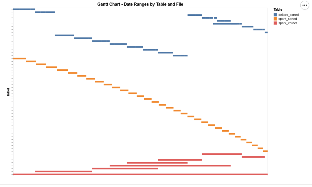
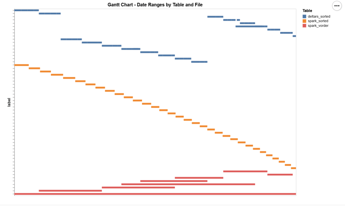
I added a bar chart to show how the data is sorted per date. As expected, Vorder is all over the place, the algorithm determines that this is the best row reordering to achieve the best RLE encoding.


The Queries

The queries are very simple. Initially, I tried more complex queries, but they involved other parts of the system and introduced more variables. I was mainly interested in testing the scan performance of VertiPaq.

Basically, it is a simple filter and aggregation.


The Test

You can download the notebook here :

def run_test(workspace, model_to_test):
    for i, dataset in enumerate(model_to_test):
        try:
            print(dataset)
            duckrun.connect(f"{ws}/{lh}.Lakehouse/{dataset}").deploy(bim_url)
            run_dax(workspace, dataset, 0, 1)
            time.sleep(300)
            run_dax(workspace, dataset, 1, 5)
            time.sleep(300)
        except Exception as e:
            print(f"Error: {e}")
    return 'done'

Deploy automatically generates a new semantic model. If it already exists, it will call clearvalue and perform a full refresh, ensuring no data is kept in memory. When running DAX, I make sure ClearCache is called.

The first run includes only one query; the second run includes five different queries. I added a 5-minute wait time to create a clearer chart of capacity usage.


Capacity Usage

To be clear, this is not a general statement, but at least in this particular case with this specific dataset, the biggest impact of Vorder seems to appear in the capacity consumption during the cold run. In other words:

Transcoding a vanilla Parquet file consumes more compute than a Vordered Parquet file.

Warm runs appear to be roughly similar.


Impact on Performance

Again, this is based on only a couple of queries, but overall, the sorted data seems slightly faster in warm runs (although more expensive). Still, 120 ms vs 340 ms will not make a big difference. I suspect the queries I ran aligned more closely with the column sorting—that was not intentional.


Takeaway

Just Vorder if you can. Make sure you enable it when starting a new project. ETL, data engineering have only one purpose, make the experience of the end users the best possible way, ETL job that take 30 seconds more is nothing compared to a slower PowerBI reports.

now if you can’t, maybe you are using a shortcut from an external engine, check your powerbi performance if it is not as good as you expect then make a copy, the only thing that matter is the end user experience.

Another lesson is that VertiPaq is not your typical OLAP engine; common database tricks do not apply here. It is a unique engine that operates entirely on compressed data. Better-RLE encoded Parquet will give you better results, yes you may have cases where the sorting align better with your queries pattern, but in the general case, Vorder is always the simplest option.

First Look at Incremental Framing in Power BI

TL;DR: Incremental framing is like CDC to RAM 🙂 It significantly improves cold-run performance of Direct Lake mode in some scenarios, there is an excellent documentation that explain everything in details

What Is Incremental Framing?

One of the most important improvements to Direct Lake mode in Power BI is incremental framing.

Power BI’s OLAP engine, VertiPaq (probably the most widely deployed OLAP engine, though many outside the Power BI world may not know it) relies heavily on dictionaries. This works well because it is a read-only database. another core trick is its ability to do calculation directly on encoded data. This makes it extremely efficient and embarrassingly fast  ( I just like this expression for some reason ).


Direct Lake Breakthrough

Direct Lake’s breakthrough is that dictionary building is fast enough to be done at runtime.

Typical workflow:

  1. A user opens a report.
  2. The report generates DAX queries.
  3. These queries trigger scans against the Delta table.
  4. VertiPaq scans only the required columns.
  5. It builds a global dictionary per column, loads the data from Parquet into memory, and executes queries.

The encoding step happens once at the start, and since BI data doesn’t usually change more that much, this model works well.


The Problem with Continuous Appends

In scenarios where data is appended frequently (e.g., every few minutes), the initial approach does not works very well. Each update requires rebuilding dictionaries and reloading all the data into RAM, effectively paying the cost of a cold run every time ( reading from remote storage will be always slower).


How Incremental Framing Fixes This

Incremental framing solves the problem by:

  • Incrementally loading new data into RAM.
  • Encoding only what’s necessary.
  • Removing obsolete Parquet data when not needed.

This substantially improves cold-run performance. Hot-run performance remains largely unchanged.


Benchmark: Australian Electricity Market

To test this feature, I used my go-to workload: the Australian electricity market, where data is appended every 5 minutes—an ideal test case.

  • Incremental framing is on by default, I turn it off using this bog
  • For benchmarking, I adapted an existing tool , Direct Lake load testing( I just changed writing the results to Delta instead of CSV), I used 8 concurrent users, the main fact Table is around 120 M records, the queries reflect a typical user session , this is a real life use case, not some theoretical benchmark.

Results

P99

P99 (the 99th percentile latency, often used to show worst-case performance):

  • Improvement of 9x–10x, again, your results may varied depending on workload, Parquet layout, and data distribution.

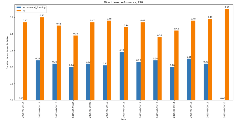
P90

P90 (90th percentile latency):

  • Less dramatic but still strong.
  • Improved from 500 ms → 200 ms.
  • Faster queries also reduce capacity unit usage.

Geomean

just for fun and to show how fast Vertipaq is, let’s see the geomean, alright went from 11 ms to 8 ms, general purpose OLAP engines are cool, but specialized Engines are just at another level !!!

This does not solve Bad Table layout problem

This feature improves support for Delta tables with frequent appends and deletes. However, performance still degrades if you have too many small Parquet row groups.

VertiPaq does not rewrite data layouts—it reads data as-is. To maintain good performance:

  • Compact your tables regularly.
  • In my case, I backfill data nightly. The small Parquets added during the day don’t cause major issues, but I still compact every 100 files as a precaution.

If your data is produced inside Fabric, VOrder helps manage this. For external engines (Snowflake, Databricks, Delta Lake with Python), you’ll need to actively manage table layout yourself.

First Look at Geometry Types in Parquet

Getting different parties in the software industry to agree on a common standard is rare. Most of the time, a dominant player sets the rules. Occasionally, however, collaboration happens organically and multiple teams align on a shared approach. Geometry types in Parquet are a good example of that.

In short: there is now a defined way to store GIS data in Parquet. Both Delta Lake and Apache Iceberg have adopted the standard ( at least the spec). The challenge is that actual implementation across engines and libraries is uneven.

  • Iceberg: no geometry support yet in Java nor Python, see spec
  • Delta:  it’s unclear if it’s supported in the  open source implementation (I need to try sedona and report back), nothing in the spec though ?
  • DuckDB: recently added support ( you need nightly build or wait for 1.4)
  • PyArrow: has included support for a few months, just use the latest release
  • Arrow rust : no support, it means, no delta python support 😦

The important point is that agreeing on a specification does not guarantee broad implementation. and even if there is a standard spec, that does not means the initial implementation will be open source, it is hard to believe we still have this situation in 2025 !!!

Let’s run it in Python Notebook

To test things out, I built a Python notebook that downloads public geospatial data, merges it with population data, writes it to Parquet, and renders a map using GeoPandas, male sure to install the latest version of duckdb, pyarrow and geopandas

!pip install -q duckdb  --pre --upgrade
!pip install -q pyarrow --upgrade
!pip install geopandas  --upgrade
import sys
sys.exit(0)

At first glance, that may not seem groundbreaking. After all, the same visualization could be done with GeoJSON. The real advantage comes from how geometry types in Parquet store bounding box coordinates. With this metadata, spatial filters can be applied directly during reads, avoiding the need to scan entire datasets.

That capability is what makes the feature truly valuable: efficient filtering and querying at scale, note that currently duckdb does not support pushing those filters, probably you need to wait to early 2026 ( it is hard to believe 2025 is nearly gone)

👉Workaround if your favorite Engine don’t support it .

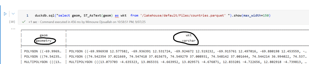
 A practical workaround is to read the Parquet file with DuckDB (or any library that supports geometry types) and export the geometry column back as WKT text. This allows Fabric to handle the data, albeit without the benefits of native geometry support, For example PowerBI can read WKT just fine

duckdb.sql("select geom, ST_AsText(geom) as wkt  from '/lakehouse/default/Files/countries.parquet' ")

For PowerBI support to wkt, I have written some blogs before, some people may argue that you need a specialized tool for Spatial, Personally I think BI tools are the natural place to display maps data 🙂