Iceberg on a single node is coming together

For a long time, whenever I tried to use Iceberg outside the JVM ecosystem, something I needed seemed to be waiting for the next release. It took longer than I hoped, but lately I have been able to get much further with the engines I use.

chDB can authenticate to OneLake with a token, Polars now runs all 22 queries in this benchmark, and DuckDB’s cache feels like absolute magic on the second pass. I still ran into bugs, but I could run both reads and writes across several engines against the same Iceberg catalog.

I took two of my notebooks and port them to GitHub Actions as python script across DuckDB, Polars, chDB, LakeSail, Spark and Daft. One runs analytical queries; the other reads CSVs and writes Iceberg tables. I wanted to see how each handled the workloads on a small 4-core runner.

The data lives in OneLake. Reading through its Iceberg REST catalog is already available; the write support I used is still in private preview.

Both benchmarks run on a public 4 vCPU / 16 GB runner. The engines connect to the catalog either directly or through pyiceberg. OIDC federation provides a token per job, so there is no client secret to store. The same approach should work with other Iceberg REST catalogs, provided the engine supports their storage and authentication.

The code, the raw JSON of every run and the charts are in djouallah/lakehouse_benchmark.

Reading: TPC-H-like queries at SF10

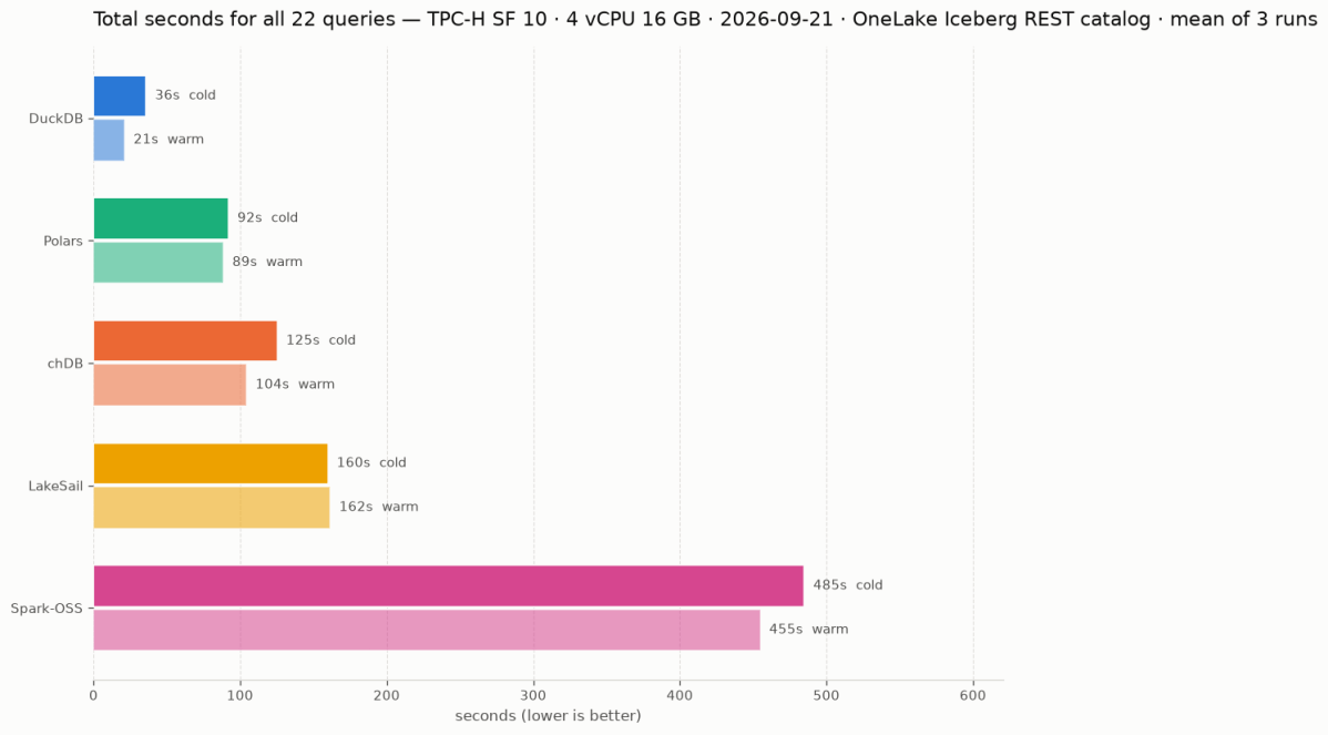
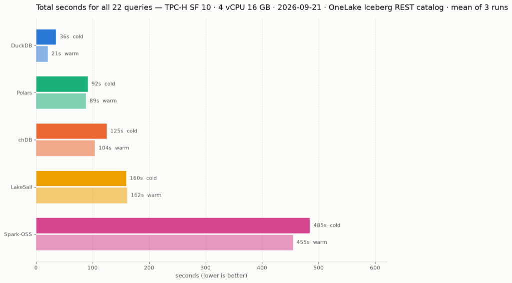
The tables are generated with tpchgen, uploaded as Parquet and registered with pyiceberg’s add_files. DuckDB and LakeSail could have written them just fine, but I wanted to stay neutral. Each engine attaches the catalog, runs the 22 queries, then runs the same 22 again immediately. Those are the cold and warm passes below; catalog attach time is excluded. The chart and the table are the mean of three runs on 20 and 21 September 2026. This is a small single-node comparison, not an official TPC-H benchmark.
EngineVersionColdWarm
DuckDB2.0.0 dev35.9s21.3s
Polars2.0.0-rc.292.1s88.6s
chDB4.4.0125.4s104.5s
LakeSail0.7.1159.9s161.6s
Spark-OSS4.1.3484.9s454.9s

Spark open source, not to be confused with Fabric Spark, is a single-node JVM on 4 cores here. Thanks to AI, running Spark locally is no longer a scary experience. Unfortunately Daft is missing: at 0.7.25 it runs 16 of the 22 queries, because l_extendedprice * (1 - l_discount) overflows its decimal precision ceiling of 38 (Daft#7532). I like Daft and would love to include it in the full query comparison once this is fixed. It does complete the ETL workload below.

Writing: Light ETL

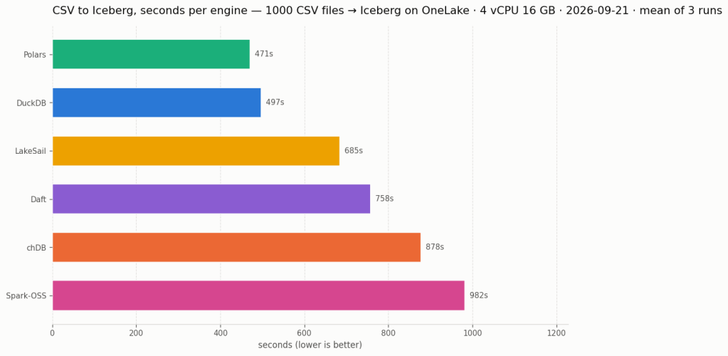
1000 daily AEMO CSV files, 52 GB, are landed once in the lakehouse Files/ section. Each engine reads all of them, filters, casts and writes one Iceberg table of 149,146,763 rows through the same catalog. DuckDB, LakeSail and Spark have their own Iceberg writer. chDB and Polars stream Arrow batches into pyiceberg. Daft has its own writer over a pyiceberg table.
EngineLoad
Polars470.8s
DuckDB497.4s
LakeSail684.5s
Daft757.9s
chDB878.1s
Spark-OSS982.2s

Every engine ends with the same row count. Load time includes recreating the table, reading the CSVs, transforming, writing and committing; session setup and catalog attach are timed separately. There is one load pass per engine, and the chart and the table are the mean of three runs. Snapshot isolation and concurrent writes will have to wait for another blog. The Iceberg write path used here is in private preview.

Random learnings, in no particular order

  • DuckDB needed AZURE_TRANSPORT_OPTION_TYPE=curl on this Linux runner. Without it the Iceberg attach succeeds and every data-file read fails with a message that looks exactly like a missing credential. Setting the transport fixed it. I had not seen this in the Fabric notebook.
  • chDB returned 41 rows for Q13, everybody else 42. ClickHouse defaults join_use_nulls=0 and fills unmatched outer-join cells with default values instead of NULL. The row-count smoke test caught this, and the benchmark now sets join_use_nulls=1.
  • The catalog cache settings do not all mean the same thing. I configured a 15-minute lifetime, but LakeSail’s “table cache” caches the table listing, not the loaded table. It still loads table metadata on every statement, adding REST requests even on the warm pass (sail#2629).
  • Daft’s six query failures come from decimal arithmetic. CTEs, EXISTS and correlated subqueries all work. It also rejects backticks outright, which looked like a total dialect failure until I read the error. Separately, its Azure URI parser drops the container on OneLake hosts; the bench works around it with az:// paths. The proposed fix is Daft#7533.
  • Nothing is partitioned, on purpose. The pyiceberg streaming append used here only supports unpartitioned tables. A first version that materialised batches to partition by year took the 16 GB runner down at 100 files. So every engine writes the same unpartitioned shape and year stays a plain column.

Spark, and why it has no native accelerator here

Spark-OSS is 4.1.3 with Iceberg 1.11 and hadoop-azure 3.4.2. I also looked at Comet and Gluten/Velox, but could not use either for this benchmark.

  • Comet supports Spark 4.1 and ships a native Iceberg reader, but its readable schemes are file, s3, s3a, gs, oss. An abfss table is declined at planning time and runs on the JVM as if the plugin were not there. I left Comet out because it could not accelerate these scans. Filed as datafusion-comet#6058.
  • Gluten/Velox has a Velox ABFS connector, but I could not find a published package for Spark 4.x to test.

Conclusion

All six engines completed the CSV-to-Iceberg load. Five completed all 22 read queries; Daft completed 16. Being able to try this many engines against one catalog, with the data staying in OneLake, is what I find exciting. chDB’s token support and Polars running all 22 SQL queries give me more options for the notebooks I already use.

DuckDB was fastest on the reads, and on the load it traded first place with Polars from run to run. DuckDB’s read total fell from 36s to 21s on the second pass, about 40%. The other engines improved less, and LakeSail’s warm pass came out slightly slower than its cold one. That makes repeated reads worth testing separately from a one-pass load. It does not tell us exactly what each engine cached or how many bytes it fetched; chDB also has a filesystem cache configured here.

For my ETL workload, I care more about the first pass: read the new files, transform them and write the table. For repeated analytics, I would also look closely at the warm timings.

If you want to see how much things have changed, have a look at these TPC-H SF10 results from four years ago.

The timings above come from the JSON under results/. To run the benchmarks against your own workspace, follow RUN.md for the Entra app registration and tenant settings. The write benchmark requires access to the private preview used here.

Writing Databricks Parquet That VertiPaq Likes

This post, the repo and every number in it are personal opinion. Nothing here is a Fabric position, benchmark or recommendation.

My colleague Eiki published a post on Microsoft’s white paper on Power BI architecture choices for Azure Databricks. Read it first: it covers the four storage modes, the headline findings, and links to the paper. I assume you know what the paper measured.

I like the paper for a different reason. It benchmarks a lakehouse as designed: open files on object storage, one vendor writes, another reads, Parquet is the only contract. Such benchmarks are rare, hard to reproduce and usually opinionated. This one is deliberately neutral (maybe too neutral) , The dataset is so uniform that V-Order has little room to differentiate the writers, so all writers start on relatively equal ground.

I have written before about VertiPaq reading Parquet that other engines wrote: Optimizing Parquet Layout for Power BI Direct Lake Mode (Dec 2024), Just VOrder, don’t try to understand how VertiPaq works (Nov 2025) and Writing Parquet That VertiPaq Likes (Aug 2026).

The short version: VertiPaq reads Parquet from any producer. It does not need V-Order. It prefers a layout it can transcode fast and hold small, and V-Order is one way to produce it.

This post applies that idea to Spark on Databricks. I am not a Spark expert; I know delta-rs much better. The Parquet concepts carry over, the knobs do not, and Databricks has many settings that interact.

AI helped me navigate them. Where the repo gets Spark wrong, the mistake is mine. Corrections welcome.

What I did

The paper tunes the Databricks write with the mainstream, documented settings, as an industry paper has to. This is a personal blog, so I can be less orthodox and go low level 🙂 I tried a few little-known knobs instead.

All of them are cluster configuration for row-group size and dictionary encoding, the same lines for every table, plus one optional step per fact table: a single clustering key on the column the reports filter on (nothing fancy it is just a global sort).

I used the paper’s protocol: TPC-DS at SF100 and SF1000, its DAX capture, 20 concurrent readers, three load tests back to back on one model. Two changes: the semantic model is deleted after the three runs so the next run starts cold, and the OneLake cache is on because my Databricks tenant is in another region. Only the very first run at a scale factor reads across regions; every later run 1 reads from the cache, so it measures the transcode alone.

Note: I used Fabric layout as it is.

Databricks writes, Direct Lake reads through the mirrored catalog. The configuration, what each line does and what breaks it are in the repo. This post is results only.

The results

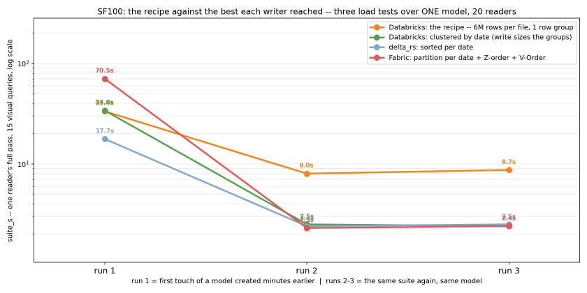
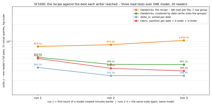
Each chart shows the configuration alone, the configuration with the clustering key, and the best layout of each other writer: delta-rs sorted on the date key, and the paper’s Fabric layout of one partition per date with Z-order and V-Order.

Run 1 pays the transcode; runs 2 and 3 rerun the same queries on the loaded model.

At SF100, the configuration alone produces dictionary encoding and large row groups, but is about three times slower than every ordered layout. Adding the clustering key on the date matches the paper’s V-Order layout, with row groups more than ten times larger.

At SF1000, the configuration alone never really warms up: each run is slower than the last, while the three ordered layouts do. That is why the clustering key is not just an optimisation in the recipe; it is what makes the layout usable at this scale. The clustered arm still trails delta-rs and the paper’s layout at SF1000: the clustering did not fully sort the rows at that scale, and the repo carries that as open. Why delta-rs has the best cold run at both scale factors is still a mystery to me.

The interesting part is that VertiPaq does not care who wrote the Parquet. It cares about the physical layout it has to transcode.

The repo

github.com/djouallah/parquet_layout_vertipaq_spark has the configuration, the clustering step, what undoes it, the numbers behind both charts and what is still open.

It also ships a Claude Code skill that applies the recipe.

Writing Parquet That VertiPaq Likes

This rabbit hole started with a simple observation: VertiPaq seemed to like parquet produced by delta-rs more than parquet produced by DuckDB — and that drove me nuts. delta-rs was at the time a niche library for nerds; Fabric didn’t even have a Python notebook. The mental model was simple: write with Spark, get V-Order, get the best possible layout for Power BI.

It is 2026; Fabric is more widespread, and there are simply more patterns and use cases:

  • New Fabric workspaces default Spark to the writeHeavy resource profile, which does not write V-Order.
  • Customers — especially on smaller SKUs — routinely write with delta-rs from Python notebooks.
  • Reading tables written by Snowflake, Databricks and BigQuery through Direct Lake is a production pattern.

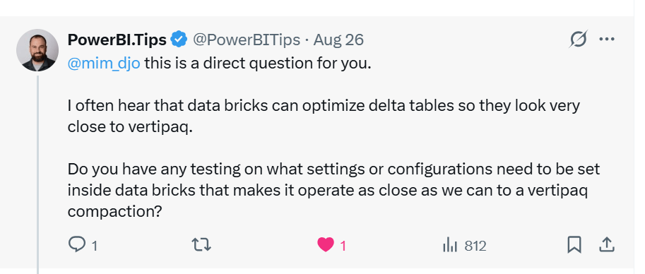
So “what parquet is friendly to Vertipaq” is now a legitimate data engineering question — I can’t tell you how happy I was when I read this tweet 🙂

The short version

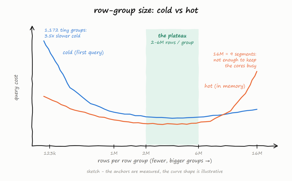
  1. Row groups of a few million rows : 2–6M rows per group; never go above 16M, VertiPaq’s segment ceiling.
  2. Dictionary-encode every column — and make the file footer say so.
  3. One global ORDER BY, lowest-cardinality columns first, date up front. No clustering, no Z-ordering, none of that.
  4. Delta vs Iceberg does not matter. Only the parquet inside the table matters.

Method

I treated VertiPaq as a black box and did what experimental science does with a phenomenon it doesn’t understand: change one variable, measure, repeat. Nothing here is confidential or internal — every number was measured from the outside, on tables anyone can rebuild.

One more thing changed this year: AI became genuinely useful for this kind of work, because it never gets bored. Sweeping writers × row-group sizes × file sizes × sort orders across hundreds of runs is exactly the tedium it doesn’t feel.

Two experiments.

  • First: figure out why VertiPaq preferred delta-rs output.
  • Second: run multiple writers and vary row-group count, file size and ordering, measuring cold, warm and hot query cost.

Caveat. Hot behaviour is well documented — after all, it is the same in-memory format as import mode — so I am more interested in cold runs (first touch of a fresh model), even though most real-world traffic is hot: a live model transcodes once and then serves from RAM.

The datasets are rather smallish — the biggest table here is around 600M rows. As a data analyst I have always dealt with small data, so I am optimising for the workload I actually care about.

How Direct Lake reads your parquet

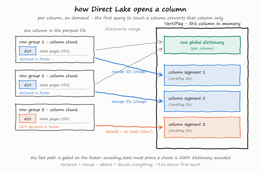
The mechanism that explains almost every finding. Transcoding is per column, on demand: the first DAX query to touch a column that is not yet in memory converts that column only into VertiPaq’s in-memory format. The column’s per-row-group parquet dictionaries are merged into one global VertiPaq dictionary, and each row group of the column is loaded as one resident column segment, remapping parquet data IDs onto VertiPaq IDs on the way in. Every query after that scans the segments the transcode produced. Query latency — and capacity consumption — is therefore a property of how the parquet was written.

Findings

Dictionary encoding is the big one

VertiPaq is itself a dictionary-based engine. When a chunk arrives dictionary-encoded, the transcode merges the parquet dictionary into the column’s global one and remaps the data IDs — it never decodes the values. Anything else has to be decoded and re-hashed, value by value, at load time. On a single 144M-row DECIMAL(18,4) column, PLAIN measured 618.6 MB against 423.1 MB dictionary-encoded — ~200 MB extra and a re-encode, on one column.

The surprise is that the encoding alone isn’t enough: the declaration is part of the encoding. The engine takes the cheap remap path only when the footer’s encoding_stats prove a chunk is entirely dictionary-encoded without decoding its pages. DuckDB’s writer emitted no encoding_stats at all until duckdb#24957 (merged 2026-08-24, currently in main only). That PR measures the cold first-touch of a 142M-row dictionary string column falling from 10,857.5 ms to 689.3 ms — about 15×, with identical pages. The attribution was verified the hard way: synthesising only that footer field into an otherwise unmodified file reproduces the speedup. A second PR, duckdb#24645 (merged 2026-08-10), adds a data_page_size_limit option — before it, DuckDB often wrote one huge data page per column chunk.

Row-group size: a tension between cold and hot

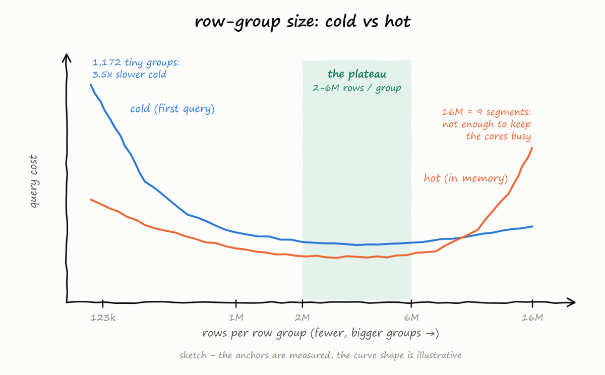
There is no single best size, but both ends fail measurably. Every row group is one more dictionary merge and one more segment to set up per column, which is why tiny groups murder the cold tier: the same DuckDB in the same notebook was 3.5× slower cold (96,503 ms vs 27,785 ms) when a library default sliced a 144M-row table into 1,172 groups of ~123k rows. At the other end, 16M rows — VertiPaq’s segment ceiling — was the worst sorted geometry measured: nine segments starve the scan pool. Cold prefers slightly bigger groups than hot, but very big groups are bad for both.

Power BI doesn’t disclose how many cores it uses, so the practical rule is: enough row groups to keep the cores busy. On the 144M-row table, warm query time stepped down between 19 and 24 groups (≈5,700 ms → 3,221 ms), and 72 groups bought nothing over 24. Hence the plateau: 2–6M rows per group.

A global sort keeps paying after the data is in memory

Transcoding does not change row order — it is essentially a working data copy into memory. So a sort applied at write time survives into the resident segments, which is why ordering matters for hot runs too, not just for compression.

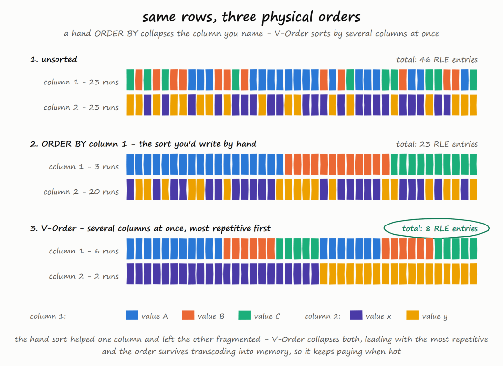
A single global ORDER BY with low-cardinality columns first (and a preference for date) produces long RLE runs. It is not V-Order — but in some cases it is good enough. When V-Order does engage, what it’s worth depends on the surface — column count × categorical skew — not row count: on a skewed 17-column taxi table it collapsed the most repetitive column to 3,371× fewer runs; on a near-unique 5-column table it left row order untouched and still shrank files 16%. One caution from the sweep: an alternative sort key cut file size a further 30% and bought statistically zero query time — sort for the columns your queries filter on, not for size on disk.

This is also the cleanest way to see what V-Order’s reorder actually is. A hand-written ORDER BY collapses the column you name and leaves the others fragmented; V-Order sorts by several columns at once, most repetitive first — the taxi measurement above is its signature, runs falling off exactly as an encoding-driven sort predicts.

VertiPaq doesn’t like ragged row groups

delta-rs closes a file the moment the size cap is hit, truncating the in-progress row group — measured writing groups at 0.43× their declared rows. A truncated group isn’t just small; it makes segment sizes uneven, exactly the non-uniform scan load you were sizing row groups to avoid. I’ve proposed a fix in delta-rs#4677 — still open, and opt-in — which rolls files only on row-group boundaries.

Dynamic row group size at write time are very hard.

I built a personal package, duckrun, using delta-rs and DuckDB and tried a clever optimisation. The plan: before writing a query’s result, estimate its row count and compute the perfect row-group size on a 1M–16M scale. It failed completely, because query planners are bad at estimating output size — DuckDB estimated ~14.9M rows for a table that actually held 143,980,961, 9.7× too low — so the “optimised” geometry was off by an order of magnitude. Derive geometry from an exact count (the table you’re rewriting, the Delta log) — never from an estimate. Not only that: in an initial version the cost of the estimation was nearly the same as writing the table 🙂

Anyway, I endup writing 6M as the default row group everywhere, i feel it is a good enough compromise

Takeaway

V-Order is usually understood as row reordering — and the reordering is real; the hard part is not the reordering itself but doing it fast (that’s the secret sauce basically), to be super clear, V-order is a local sort, not global

But it is not only that: a V-Order write also sets the row-group geometry and runs the encoding pass, keeping a declared dictionary on every column.

Two consequences follow:

 If you write with a Fabric engine, turning V-Order on is a no-brainer, and honestly, it should be the default in my personal opinion.

measured here at ~8% of build compute for up to 2.8× less query capacity (1,332 vs 3,769 CU on identical data) — the write premium is paid once, while queries pay every day. I do wish it were simpler to turn on: changing the Spark write profile is not obvious, and a lot of users don’t even know it is there. As someone who used VertiPaq for more than a decade with zero knowledge of columnar data structures, I suspect there must be a better way.

If you write with anything else — Snowflake, Databricks, delta-rs, DuckDB — my hope is that there will be more public specifications on how to optimize parquet layout for VertiPaq.

Thanks to Krystian Sakowski for answering my silly questions 🙂

Links

The Enterprise Context Layer

Edit : I vibe coded one, so you dont need to read this whole text

https://djouallah.github.io/fabric-context-layer

As a data analyst, I have been following the progress of LLMs in analytics, and although there has been some progress in accuracy and in the kinds of questions you can ask, overall, it hasn’t had the impact I was hoping for. That’s a totally different story for coding and data engineering, where AI is already changing daily workflows. The core idea is simple: if something is falsifiable, AI can be useful.

In the last couple of months, I keep hearing about some new terms which I never really understood: knowledge graphs, ontology (Andre, who is someone I respect a lot calls it the Enterprise brain), and so on. But I think there may be something genuinely interesting here for analytics.

There is so much data in an enterprise, and so much of it is still underused. Talking about a context layer is not new, and there is plenty of literature on it, but it is rare to see it from the end user perspective.

There are mainly two approaches. One requires modelling, which instinctively bothers me because it expects me to do more work upfront. Maybe it is an age thing, but I am not particularly excited about learning a new mental model. I have been doing semantic modelling for nearly a decade and I am quite happy with it.

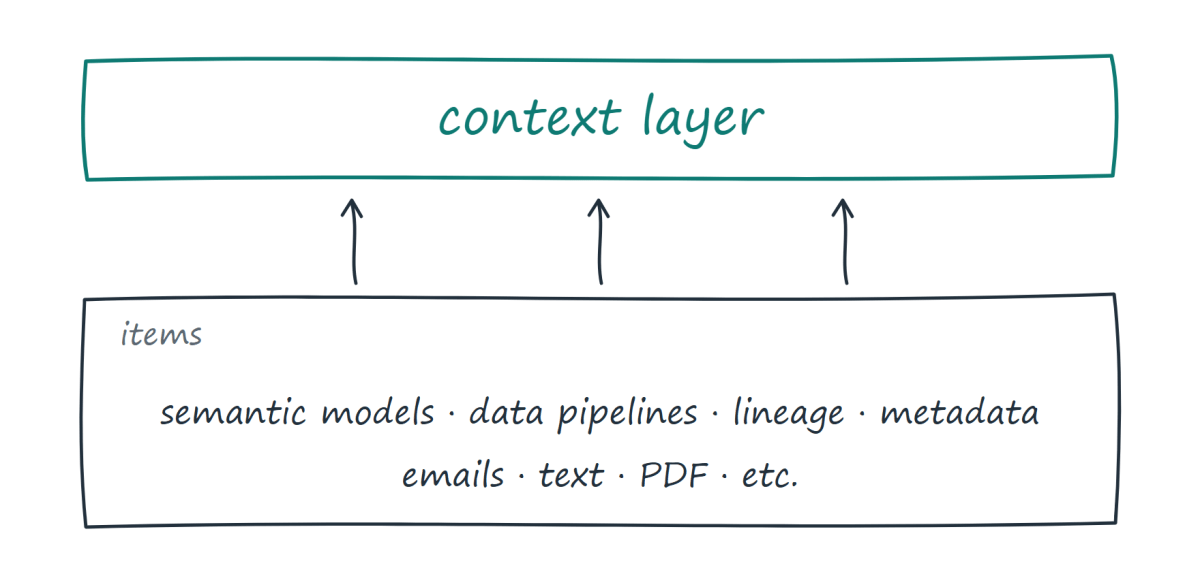
The other approach is more interesting to me because it doesn’t ask users to create something new. It works with what they already have: semantic models, data pipelines, the data itself, unstructured data, PDFs, folders, and so on. It figures out what already exists and how the pieces relate to each other. When you ask a question, it helps route you to the right place.

There is no magic here. To get a correct answer, you still need the hard work that has already been done: good semantic modelling, good metadata, good data, and so on.

For me, a system that can simply pick the right dashboard to use is already extremely useful. In a data platform, sometimes we don’t even know where to ask a question or which dashboard is more useful than another, unless we ask an analyst or a colleague. In a sense, this is just formalising what already happens in real life.

Even if the system says, “This is the question people are asking, and I don’t know of a good answer,” that’s already very useful feedback for analysts.

And one may argue, what if two semantic models authored by different departments don’t have the same definition? A naive answer would be to create one giant semantic model that unifies everything, which will never happen because this is fundamentally a human and organisational problem, not a technical one.

Maybe the better approach is simply to formalise what we already do today. Whatever the CEO, manager, or wider organisation is actually using probably makes more sense to prioritise, regardless of whether it is objectively the truth. We can imagine the system using signals: a certified dataset might carry more weight, or perhaps the author of a dataset has more credibility.

This is not a problem specific to analytics. Ask two news channels to describe the same event and you will often get different interpretations.

But to be super clear, the numbers themselves should never be non-deterministic. The measures are authored in exisitng semantic models, not made up on the fly

The bigger idea is that the context could improve with usage. Data platforms already have an enormous amount of telemetry. They know who uses what, which reports are popular, which datasets are trusted, and which questions people keep asking. There is nothing particularly new about this data. What is new is the possibility of using it to help both agents and humans find answers based on what the organisation actually uses and trusts.

In other words, the context isn’t something you build once and then leave alone. It could continuously evolve based on how the organisation actually works.

Users, I think, will not care how those signals are calculated. Users are selfish (speaking for myself here) and care only whether it is useful or not. Companies may want a say in what gets prioritised and how it works, or they may want to export that knowledge somewhere else. But I suspect they will mostly be happy if it just works.

I think the reason this may work now is that AI is becoming good enough for a lot of things. What it needs is not necessarily more intelligence, but better grounding in the knowledge that already exists inside an organisation.

I came from the construction industry, and we had this thing called delay analysis. It is basically an attempt to prove that a project delay is not the contractor’s fault. Maybe the client kept changing requirements, failed to approve drawings on time, or introduced other changes that affected the schedule.

Companies spend a lot of money on consultants who come in, read thousands of documents and pieces of correspondence, and try to rebuild a simplified model of what happened.

I know this is a very specific example, but I think AI should be able to solve this surprisingly well.

I can imagine a data platform where a supervisor asks, “What’s going on? Why are we late?” and gets an answer based on the actual project data, with references to the relevant dashboard, emails, RFIs, documents, and other evidence.

That is the kind of thing I would pay money for.

Maybe that’s what an enterprise context layer really is: not another model people have to maintain, but a way of making the knowledge an organisation already has actually useful. I am not saying this is a solved problem, or even that it will work in practice, but I think it is something worth building.