I’ve been following the evolution of Iceberg shortcuts to OneLake and I’m genuinely impressed with how the engineering team has invested so much energy into making it more robust, it is a good idea to read the documentation.
Essentially, XTable is used behind the scenes. Think of it as a translator for your open table format. Instead of requiring you to convert data from one format (like Iceberg) to another (like Delta) just to query them together, XTable allows you to access and interact with tables in different formats as if they were a single, unified table within OneLake—all without user intervention.
To truly put this to the test, I recently ran an experiment in a real production environment using my paid tenant—no sandboxes here! Here’s the logic from the Python notebook:
Accessing data from an Iceberg table using a shortcut (sourced from Snowflake; the data can be stored anywhere—Azure, S3, GCP, or OneLake, You can use BigQuery too or any Iceberg writer).
Inserting arbitrary data and performing delete operations.
Counting the total rows using Snowflake.
Counting the total rows using Fabric notebook as a Delta Table.
Recording the record counts in a results table to track and visualize the comparison over time.
The results were quite awesome. I plotted the total record counts from both the Iceberg and Delta perspectives using two distinct colors and observed a perfect match. This confirms the seamless interoperability provided by XTable.
Lesson learned:
See the code snippet below for inserting data in Snowflake:
snow.execute(f'insert into ONELAKE.ICEBERG.scada select * from ONELAKE.AEMO.SCADARAW limit {limit};')
snow.execute('delete from ONELAKE.ICEBERG.scada where INITIALMW = 0')
snow.execute("SELECT SYSTEM$GET_ICEBERG_TABLE_INFORMATION('ONELAKE.iceberg.scada');")
In rare cases—especially when running multiple transactions at the same time—Snowflake may not instantly generate the metadata. To be 100% sure, run this SQL statement
to force the engine to write new Iceberg metadata. It’s an annoying aspect of Iceberg: every commit generates three files. That’s a bit excessive. Some engines prefer to group multiple commits to reduce the size of the metadata. Again, it’s rare—but it does happen.
Note: The blog and especially the code were written with the assistance of an LLM.
TL;DR
I built a simple Fabric Python notebook to orchestrate sequential SQL transformation tasks in OneLake using DuckDB and delta-rs. It handles task order, stops on failure, fetches SQL from external sources (like GitHub or a Onelake folder), manages Delta Lake writes, and uses Arrow recordbacth for efficient data transfer, even for large datasets. This approach helps separate SQL logic from Python code and simulates external table behavior in DuckDB. Check out the code on GitHub: https://github.com/djouallah/duckrun
pip install duckrun
Introduction
Inspired by tools like dbt and sqlmesh, I started thinking about building a simple SQL orchestrator directly within a Python notebook. I was showing a colleague a Fabric notebook doing a non-trivial transformation, and although it worked perfectly, I noticed that the SQL logic and Python code were mixed together – clear to me, but spaghetti code to anyone else. With Fabric’s release of the user data function, I saw the perfect opportunity to restructure my workflow:
Data ingestion using a User-Defined Function (UDF), which runs in a separate workspace.
Data transformation in another workspace, reading data from the ingestion workspace as read-only.
All transformations are done in pure SQL, there 8 tables, every table has a sql file, I used DuckDB, but feel free to use anything else that understands SQL and output arrow (datafusion, chdb, etc).
Built Python code to orchestrate the transformation steps.
PowerBI reports are in another workspace
I think this is much easier to present 🙂
I did try yato, which is a very interesting orchestrator, but it does not support parquet materialization
How It Works
The logic is pretty simple, inspired by the need for reliable steps:
Your Task List: You provide the function with a list (tasks_list). Each item has table_name (same SQL filename, table_name.sql) and how to materilize the data in OneLake (‘append’ , ‘overwrite’,ignore and None)
Going Down the List: The function loops through your tasks_list, taking one task at a time.
Checking Progress: It keeps track of whether the last task worked out using a flag (like previous_task_successful). This flag starts optimistically as True.
Do or Don’t: Before tackling the current task, it checks that flag.
If the flag is True, it retrieves the table_name and mode from the current task entry and passes them to another function, likely called run_sql. This function performs the actual work of running your transformation SQL and writing to OneLake.
If the flag is False, it knows something went wrong earlier, prints a quick “skipping” message, and importantly, uses a break statement to exit the loop immediately. No more tasks are run after a failure.
Updating the Status: After run_sql finishes, run_sql_sequence checks if run_sql returned 1 (our signal for success). If it returns 1, the previous_task_successful flag stays True. If not, the flag flips to False.
Wrap Up: When the loop is done (either having completed all tasks or broken early), it prints a final message letting you know if everything went smoothly or if there was a hiccup.
The run_sql function is the workhorse called by run_sql_sequence. It’s responsible for fetching your actual transformation SQL (that SELECT … FROM raw_table). A neat part here is that your SQL files don’t have to live right next to your notebook; they can be stored anywhere accessible, like a GitHub repository, and the run_sql function can fetch them. It then sends the SQL to your DuckDB connection and handles the writing part to your target OneLake table using write_deltalake for those specific modes. It also includes basic error checks built in for file reading, network stuff, and database errors, returning 1 if it succeeds and something else if it doesn’t.
You’ll notice the line con.sql(f””” CREATE or replace SECRET onelake … “””) inside run_sql; this is intentionally placed there to ensure a fresh access token for OneLake is obtained with every call, as these tokens typically have a limited validity period (around 1 hour), keeping your connection authorized throughout the sequence.
When using the overwrite mode, you might notice a line that drops DuckDB view (con.sql(f’drop VIEW if exists {table_name}’)). This is done because while DuckDB can query the latest state of the Delta Lake files, the view definition in the current session needs to be refreshed after the underlying data is completely replaced by write_deltalake in overwrite mode. Dropping and recreating the view ensures that subsequent queries against this view name correctly point to the newly overwritten data.
The reason we do this kind of hacks is, duckdb does not support external table yet, so we are just simulating the same behavior by combining duckdb and delta rs, spark obviousely has native support
Handling Materialization in Python
One design choice here is handling the materialization strategy (whether to overwrite or append data) within the Python code (run_sql function) rather than embedding that logic directly into the SQL scripts.
Why do it this way?
Consider a table like summary. You might have a nightly job that completely recalculates and overwrites the summary table, but an intraday job that just appends the latest data. If the overwrite or append command was inside the SQL script itself, you’d need two separate SQL files for the exact same transformation logic – one with CREATE OR REPLACE TABLE … AS SELECT … and another with INSERT INTO … SELECT ….
By keeping the materialization mode in the Python run_sql function and passing it to write_deltalake, you can use the same core SQL transformation script for the summary table in both your nightly and intraday pipelines. The Python code dictates how the results of that SQL query are written to the Delta Lake table in OneLake. This keeps your SQL scripts cleaner, more focused on the transformation logic itself, and allows for greater flexibility in how you materialize the results depending on the context of your pipeline run.
Efficient Data Transfer with Arrow Record batch
A key efficiency point is how data moves from DuckDB to Delta Lake. When DuckDB executes the transformation SQL, it returns the results as an Apache Arrow RecordBatch. Arrow’s columnar format is highly efficient for analytical processing. Since both DuckDB and the deltalake library understand Arrow, data transfers with minimal overhead. This “zero-copy” capability is especially powerful for handling datasets larger than your notebook’s available RAM, allowing write_deltalake to process and write data efficiently without loading everything into memory at once.
Example:
you pass Onelake location, schema and the number of files before doing any compaction
first it will load all the existing Delta table
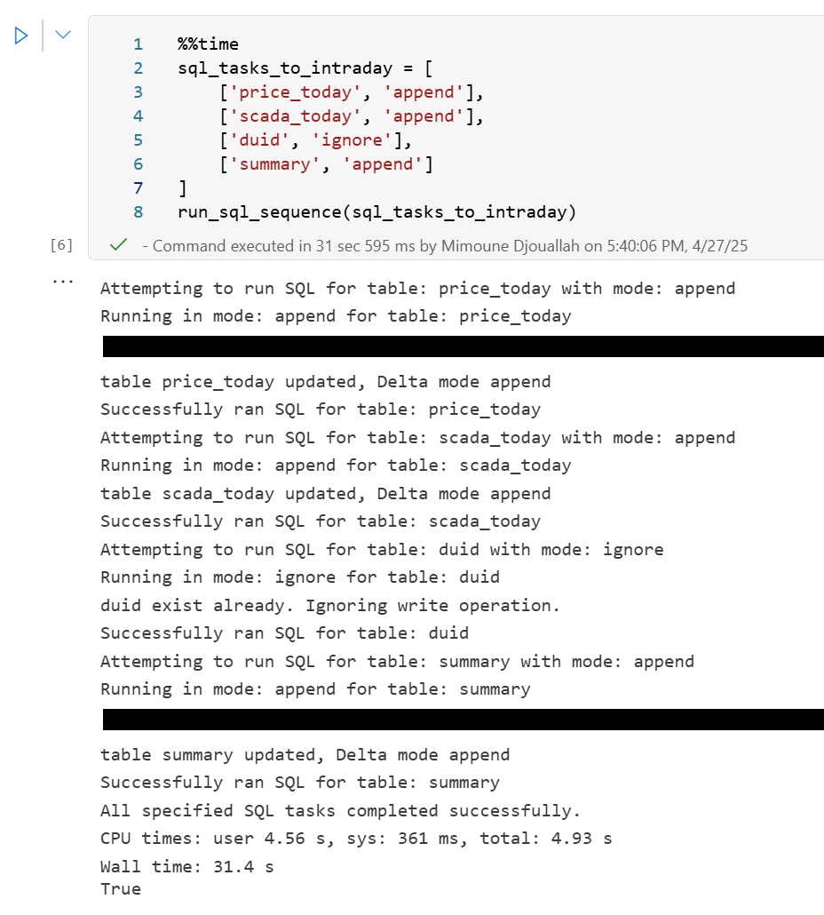
Here’s an example showing how you might define and run different task lists for different scenarios:
sql_tasks_to_intraday = [ ['price_today', 'append'], ['scada_today', 'append'], ['duid', 'ignore'], ['summary', 'append'] # Append to summary intraday using the *same* SQL script ]
You can then use Python logic to decide which pipeline to run based on conditions, like the time of day:
start = time(4, 0)
end = time(5, 30)

if start <= now_brisbane <= end:
    run_sql_sequence(sql_tasks_to_run_nightly)
Here’s an example of an error I encountered during a run, it will automatically stop the remaining tasks:
Attempting to run SQL for table: price_today with mode: append
Running in mode: append for table: price_today
Error writing to delta table price_today in mode append: Parser Error: read_csv cannot take NULL list as parameter
Error updating data or creating view in append mode for price_today: Parser Error: read_csv cannot take NULL list as parameter
Failed to run SQL for table: price_today. Stopping sequence.
One or more SQL tasks failed.
here is some screenshots from actual runs
as it is a delta table, I can use SQL endpoints to get some stats
For example the table scada has nearly 300 Million rows, the raw data is around 1 billion of gz.csv
It took nearly 50 minutes to process using 2 cpu and 16 GB of RAM, notice although arrow is supposed to be zero copy, writing parquet directly from Duckdb is substantially faster !!! but anyway, the fact it works at all is a miracle 🙂
in the summary table we remove empty rows and other business logic, which reduce the total size to 119 Million rows.
here is an example report using PowerBI direct lake mode, basically reading delta directly from storage
In this run, it did detect that the the night batch table has changed
Conclusion
To be clear, I am not suggesting that I did anything novel, it is a very naive orchestrator, but the point is I could not have done it before, somehow the combination of open table table format, robust query engines and an easy to use platform to run it make it possible and for that’s progress !!!
I am very bad at remembering python libraries syntax but with those coding assistants, I can just focus on the business logic and let the machine do the coding. I think that’s good news for business users.
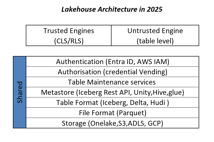
This is more or less the industry consensus on how a Lakehouse architecture should look in 2025.
By now, it’s become clear that Parquet is the de facto standard for storing data, and using an object store to separate storage from compute makes a lot of sense.
Another interesting development is how vendors want to package this offering. Storage vendors saw an opportunity to do more—after all, there’s no law that says the metastore belongs to the data warehouse! So you get things like S3 Table and Cloudflare R2, which I think is a good thing, especially if you’re a smaller analytics vendor. Life becomes much easier when table maintenance is done upstream, allowing you to focus solely on making the query engine faster.
Encouraging things are also happening in the table format space. I know a bit about Iceberg and Delta, but not much about the others. One very interesting development is Iceberg adopting deletion vectors from Delta in the V3 spec, while Delta will requires a catalog for read and write (at least for catalog managed table). I like to call it the “Icebergification” of Delta.
Another trend is the Delta Java writer making it easier to auto-generate Iceberg metadata. and Xtable is doing the same regardless of the delta writer, At this stage, one could argue: why do we need two table formats that are becoming virtually identical?
Data Analyst—How About Me?
These improvements mostly impact the write path, which is primarily managed by data engineers. But what about data analysts and end users?
if you have Fabric OneLake, you can use Direct Lake in OneLake mode. Marco has a great article about it. It’s a fantastic improvement compared to the initial version of Direct Lake. However, it doesn’t solve the problem if your data is hosted in an S3 table or BigQuery Iceberg table. Yes, you can create a shortcut to OneLake and read it from there, but that still depends on a data engineer setting it up.
Now imagine a world where an Excel, Tableau, or Power BI Desktop user (or any arbitrary client tool) can just point to a Lakehouse using a standard API, discover tables, read data, and build reports. Honestly, this isn’t a big ask , we already have this when connecting to databases using ODBC, and I don’t see any technical reason why we can’t have the same experience with Lakehouses.
We Already Have This API
For me, the most promising development in the Lakehouse ecosystem is the Iceberg Catalog REST API, and I genuinely hope it becomes a standard—just like ODBC is today (and hopefully ADBC in the future, but that’s another topic).
Again, speaking as a data analyst, I want my tools to support the read part of the API—just the ability to list tables and scan a table. That’s all. I have zero interest in how the data is stored or which table format is used. The catalog should be smart enough to generate metadata on the fly.
The Good News
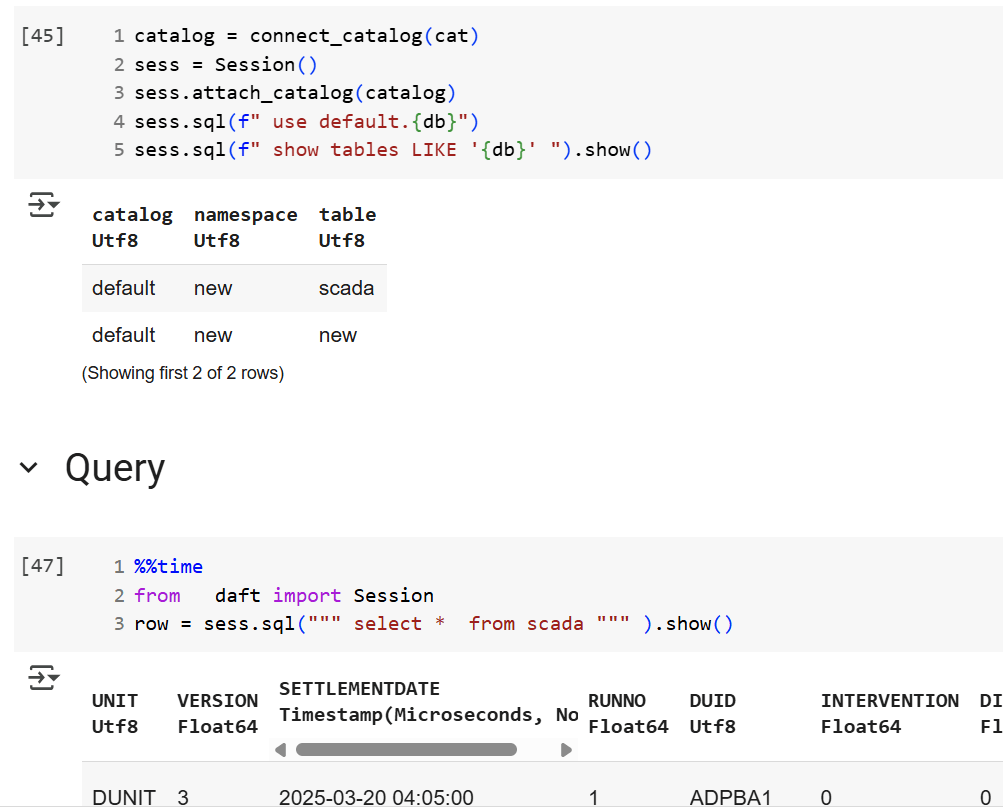
We’re getting there—at least if you’re using a Python notebook. Here’s an example where I use the same Iceberg REST API to query a table from four different Lakehouse implementations using Daft.
def connect_catalog(cat):
  match cat:
    case 'polaris':
      catalog = load_catalog(
              'default',
              uri= polaris_endpoint,
              warehouse='dwh',
              scope = 'PRINCIPAL_ROLE:data_engineer' ,
              credential= polaris_key
            )
    case 's3':
      catalog = load_catalog(
              'default',
              **{
                "type": "rest",
                "warehouse": s3_warehouse ,
                "uri": "https://s3tables.us-east-2.amazonaws.com/iceberg",
                "rest.sigv4-enabled": "true",
                "rest.signing-name": "s3tables",
                "rest.signing-region": "us-east-2"
              }
            )
    case 'uc':
      catalog = load_catalog(
               'default',
              token = token ,
              uri = endpoint,
              warehouse = 'ne'
              )
    case 'r2':
      catalog = RestCatalog(
              name = 'default',
              token = token_r2 ,
              uri = endpoint_r2,
              warehouse = r2_warehouse
              )
  return catalog
Then, I run a standard SQL query using Daft SQL.
Final Thoughts
It took Parquet a decade to become a standard. We may or may not have a single standard table format—and maybe we don’t need one. But if we want this Lakehouse vision to become mainstream, then everyone should support the Iceberg Catalog REST API, at least for read operations.
DeltaProtocolError: The table has set these reader features: {'deletionVectors'} but these are not yet supported by the deltalake reader.
Alternative: Using DuckDB
A simple alternative is to use DuckDB:
import duckdb

duckdb.sql("SELECT COUNT(*) FROM delta_scan('/lakehouse/default/Tables/xxx')")
Tested with a file that contains Deletion vectors
Column Mapping
The same approach applies to column mapping as well.
Upgrading DuckDB
Currently, Fabric Notebook comes preinstalled with DuckDB version 1.1.3. To use the latest features, you need to upgrade to the latest stable release (1.2.1) :
Note: Installing packages using %pip install does not restart the kernel when you run the notebook , you need to use sys.exit(0) to apply the changes, as some packages may already be loaded into memory.
import duckdb
duckdb.sql(" force install delta from core_nightly ")
duckdb.sql(" from delta_scan('/lakehouse/default/Tables/dbo/evolution_column_change') ")
The Future of Delta Rust .
Currently, there are two Rust-based implementations of Delta:
Delta_rs: The first and more mature implementation, developed by the community. It is an independent implementation of the Delta protocol and utilizes DataFusion and PyArrow (which will soon be deprecated) as its engine. However, Delta_rs does not support deletion vectors or column mapping, though it does support writing Delta tables.
Delta Kernel_rs: The newer, “official” implementation of Delta, providing a low-level API for query engines. It is currently being adopted by DuckDB ( and Clickhouse apparently) with more engines likely to follow. However, it is still a work in progress and does not yet support writing.
There are ongoing efforts to merge Delta_rs with Delta Kernel_rs to streamline development and reduce duplication of work.
Note : although they are written in Rust, we mainly care about the Python API 🙂
Conclusion
At least for now, in my personal opinion, the best approach is to: