This is not an official Microsoft benchmark, just my personal experience.
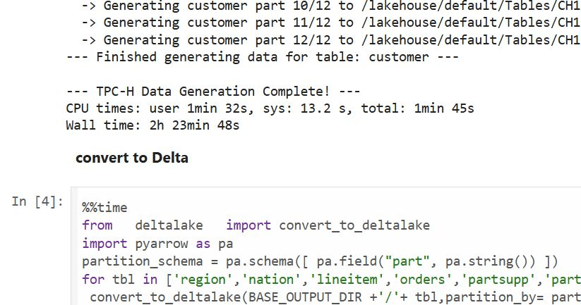
Last week, I came across a new TPCH generator written in Rust. Luckily, someone ported it to Python, which makes generating large datasets possible even with a small amount of RAM. For example, it took 2 hours and 30 minutes to generate a 1 TB scale dataset using the smallest Fabric Python notebook (2 cores and 16 GB of RAM).
Having the data handy, I tested Fabric DWH and SQL Endpoint. I also tested DuckDB as a sanity check. To be honest, I wasn’t sure what to expect.
I ran the test 30 times over three days, I think I have enough data to say something useful,In this blog, I will focus only on the results for the cold and warm runs, along with some observations.
For readers unfamiliar with Fabric, DWH and SQL Endpoint refer to the same distributed SQL engine. With DWH, you ingest data that is stored as a Delta table (which can be read by any Delta reader). With SQL Endpoint, you query external Delta tables written by Spark and other writers (this is called a Lakehouse table). Both use Delta tables.
Notes:
All the runs are using a Python notebook
to send queries to DWH/SQL Endpoint, all you need is conn = notebookutils.data.connect_to_artifact("data") conn.query("select 42")
I did not include the cost of ingestion for the DWH
The cost include compute and storage transaction and assume pay as you go rate of 0.18 $/Cu(hour)
For extracting Capacity usage, I used this excellent blog
Cold Run
The first-ever run on SQL Endpoint incurs an overhead, apparently the system build statistics. This overhead happened only once across all tests.
Point 2 is an outlier but an interesting one 🙂
The number of dots displayed is less than the number of tests runs as some tests perfectly match, which is a good sign that the system is predictable !!!
vorderimproves performance for both SQL Endpoint and DuckDB. The data was generated by Rust and rewritten using Spark; it seems to be worth the effort.
Costs are roughly the same for DWH and SQL Endpoint when the Delta is optimized by vorder, but DWH is still faster.
DuckDB, running in a Python notebook with 64 cores, is the cheapest (but the slowest). Query 17 did not run , so that result is moot. ,Still, it’s a testament to the OneLake architecture: third-party engines can perform well without any additional Microsoft integration. Lakehouse for the win.
Warm Run
vorder is better than vanilla Parquet.
DWH is faster and a bit cheaper than SQL Endpoint.
DuckDB behavior is a bit surprising, was expecting better performance , considering the data is already loaded into RAM.
Impact on the Parquet Writer
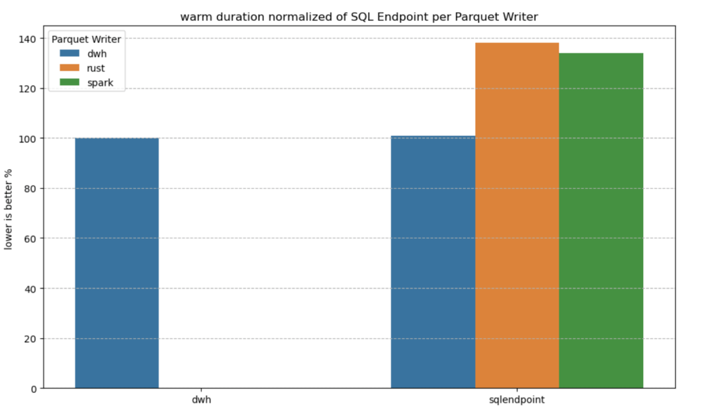
I added a chat showing the impact of using different writers on the read performance, I use only warm run to remove the impact of the first run ever as it does not happen in the DWH ( as the data was ingested)
given the same table layout, DWH and SQL Endpoint perform the same, it is expected as it is the same engine
surprisingly using the initial raw delta table vs spark optimize write gave more or less the same performance at least for this particular workload.
Final Thoughts
Running the test was a very enjoyable experience, and for me, that’s the most important thing. I particularly enjoyed using Python notebooks to interact with Fabric DWH. It makes a lot of sense to combine a client-server distributed system with a lightweight client that costs very little.
There are new features coming that will make the experience working with DWH even more streamlined.
Edit :
update the figures for Dcukdb as Query 17 runs but you need to limit the memory manually set memory_limit='500GB'
added a graph on the impact of the parquet layout.
Note: The blog and especially the code were written with the assistance of an LLM.
TL;DR
I built a simple Fabric Python notebook to orchestrate sequential SQL transformation tasks in OneLake using DuckDB and delta-rs. It handles task order, stops on failure, fetches SQL from external sources (like GitHub or a Onelake folder), manages Delta Lake writes, and uses Arrow recordbacth for efficient data transfer, even for large datasets. This approach helps separate SQL logic from Python code and simulates external table behavior in DuckDB. Check out the code on GitHub: https://github.com/djouallah/duckrun
pip install duckrun
Introduction
Inspired by tools like dbt and sqlmesh, I started thinking about building a simple SQL orchestrator directly within a Python notebook. I was showing a colleague a Fabric notebook doing a non-trivial transformation, and although it worked perfectly, I noticed that the SQL logic and Python code were mixed together – clear to me, but spaghetti code to anyone else. With Fabric’s release of the user data function, I saw the perfect opportunity to restructure my workflow:
Data ingestion using a User-Defined Function (UDF), which runs in a separate workspace.
Data transformation in another workspace, reading data from the ingestion workspace as read-only.
All transformations are done in pure SQL, there 8 tables, every table has a sql file, I used DuckDB, but feel free to use anything else that understands SQL and output arrow (datafusion, chdb, etc).
Built Python code to orchestrate the transformation steps.
PowerBI reports are in another workspace
I think this is much easier to present 🙂
I did try yato, which is a very interesting orchestrator, but it does not support parquet materialization
How It Works
The logic is pretty simple, inspired by the need for reliable steps:
Your Task List: You provide the function with a list (tasks_list). Each item has table_name (same SQL filename, table_name.sql) and how to materilize the data in OneLake (‘append’ , ‘overwrite’,ignore and None)
Going Down the List: The function loops through your tasks_list, taking one task at a time.
Checking Progress: It keeps track of whether the last task worked out using a flag (like previous_task_successful). This flag starts optimistically as True.
Do or Don’t: Before tackling the current task, it checks that flag.
If the flag is True, it retrieves the table_name and mode from the current task entry and passes them to another function, likely called run_sql. This function performs the actual work of running your transformation SQL and writing to OneLake.
If the flag is False, it knows something went wrong earlier, prints a quick “skipping” message, and importantly, uses a break statement to exit the loop immediately. No more tasks are run after a failure.
Updating the Status: After run_sql finishes, run_sql_sequence checks if run_sql returned 1 (our signal for success). If it returns 1, the previous_task_successful flag stays True. If not, the flag flips to False.
Wrap Up: When the loop is done (either having completed all tasks or broken early), it prints a final message letting you know if everything went smoothly or if there was a hiccup.
The run_sql function is the workhorse called by run_sql_sequence. It’s responsible for fetching your actual transformation SQL (that SELECT … FROM raw_table). A neat part here is that your SQL files don’t have to live right next to your notebook; they can be stored anywhere accessible, like a GitHub repository, and the run_sql function can fetch them. It then sends the SQL to your DuckDB connection and handles the writing part to your target OneLake table using write_deltalake for those specific modes. It also includes basic error checks built in for file reading, network stuff, and database errors, returning 1 if it succeeds and something else if it doesn’t.
You’ll notice the line con.sql(f””” CREATE or replace SECRET onelake … “””) inside run_sql; this is intentionally placed there to ensure a fresh access token for OneLake is obtained with every call, as these tokens typically have a limited validity period (around 1 hour), keeping your connection authorized throughout the sequence.
When using the overwrite mode, you might notice a line that drops DuckDB view (con.sql(f’drop VIEW if exists {table_name}’)). This is done because while DuckDB can query the latest state of the Delta Lake files, the view definition in the current session needs to be refreshed after the underlying data is completely replaced by write_deltalake in overwrite mode. Dropping and recreating the view ensures that subsequent queries against this view name correctly point to the newly overwritten data.
The reason we do this kind of hacks is, duckdb does not support external table yet, so we are just simulating the same behavior by combining duckdb and delta rs, spark obviousely has native support
Handling Materialization in Python
One design choice here is handling the materialization strategy (whether to overwrite or append data) within the Python code (run_sql function) rather than embedding that logic directly into the SQL scripts.
Why do it this way?
Consider a table like summary. You might have a nightly job that completely recalculates and overwrites the summary table, but an intraday job that just appends the latest data. If the overwrite or append command was inside the SQL script itself, you’d need two separate SQL files for the exact same transformation logic – one with CREATE OR REPLACE TABLE … AS SELECT … and another with INSERT INTO … SELECT ….
By keeping the materialization mode in the Python run_sql function and passing it to write_deltalake, you can use the same core SQL transformation script for the summary table in both your nightly and intraday pipelines. The Python code dictates how the results of that SQL query are written to the Delta Lake table in OneLake. This keeps your SQL scripts cleaner, more focused on the transformation logic itself, and allows for greater flexibility in how you materialize the results depending on the context of your pipeline run.
Efficient Data Transfer with Arrow Record batch
A key efficiency point is how data moves from DuckDB to Delta Lake. When DuckDB executes the transformation SQL, it returns the results as an Apache Arrow RecordBatch. Arrow’s columnar format is highly efficient for analytical processing. Since both DuckDB and the deltalake library understand Arrow, data transfers with minimal overhead. This “zero-copy” capability is especially powerful for handling datasets larger than your notebook’s available RAM, allowing write_deltalake to process and write data efficiently without loading everything into memory at once.
Example:
you pass Onelake location, schema and the number of files before doing any compaction
first it will load all the existing Delta table
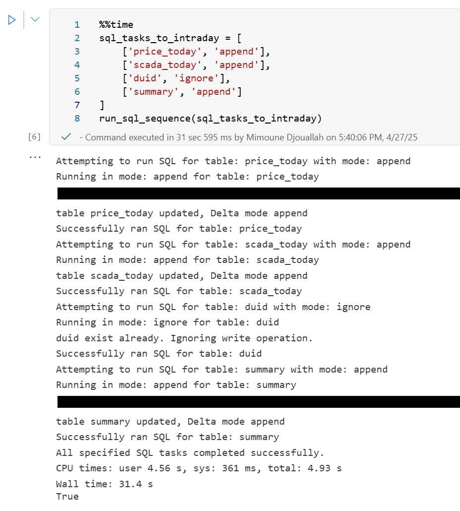
Here’s an example showing how you might define and run different task lists for different scenarios:
sql_tasks_to_intraday = [ ['price_today', 'append'], ['scada_today', 'append'], ['duid', 'ignore'], ['summary', 'append'] # Append to summary intraday using the *same* SQL script ]
You can then use Python logic to decide which pipeline to run based on conditions, like the time of day:
start = time(4, 0)
end = time(5, 30)

if start <= now_brisbane <= end:
    run_sql_sequence(sql_tasks_to_run_nightly)
Here’s an example of an error I encountered during a run, it will automatically stop the remaining tasks:
Attempting to run SQL for table: price_today with mode: append
Running in mode: append for table: price_today
Error writing to delta table price_today in mode append: Parser Error: read_csv cannot take NULL list as parameter
Error updating data or creating view in append mode for price_today: Parser Error: read_csv cannot take NULL list as parameter
Failed to run SQL for table: price_today. Stopping sequence.
One or more SQL tasks failed.
here is some screenshots from actual runs
as it is a delta table, I can use SQL endpoints to get some stats
For example the table scada has nearly 300 Million rows, the raw data is around 1 billion of gz.csv
It took nearly 50 minutes to process using 2 cpu and 16 GB of RAM, notice although arrow is supposed to be zero copy, writing parquet directly from Duckdb is substantially faster !!! but anyway, the fact it works at all is a miracle 🙂
in the summary table we remove empty rows and other business logic, which reduce the total size to 119 Million rows.
here is an example report using PowerBI direct lake mode, basically reading delta directly from storage
In this run, it did detect that the the night batch table has changed
Conclusion
To be clear, I am not suggesting that I did anything novel, it is a very naive orchestrator, but the point is I could not have done it before, somehow the combination of open table table format, robust query engines and an easy to use platform to run it make it possible and for that’s progress !!!
I am very bad at remembering python libraries syntax but with those coding assistants, I can just focus on the business logic and let the machine do the coding. I think that’s good news for business users.
While testing the DuckDB ODBC driver, which is getting better and better (not production ready but less broken compared to two years ago), I noticed something unexpected. Running queries through Power BI in DirectQuery mode was actually faster than executing them directly in the DuckDB native UI.
Naturally, that does not make sense !!!
What followed was an investigation that turned into a fun and insightful deep dive into text-to-SQL generation, Power BI’s query behavior, and the enduring relevance of manual SQL tuning
🧩 The Goal: Find the Worst Product by Return Rate
The task was straightforward:
Calculate total sales, total returns, and return rate by product. Rank the products and find the top 5 with the highest return rates.
To make it interesting, I decided to try:
Letting an LLM generate the SQL by loading the semantic model.
Using PowerBI in Direct Query Mode.
Finally, manually tuning the query.
📝 Step 1: LLM-generated SQL — Clean and Understandable
chatgpt generated a good starting point:
WITH sales_by_product AS   (
    SELECT
        i.i_product_name AS product_name,
        SUM(ss.ss_sales_price * ss.ss_quantity) AS total_sales
    FROM store_sales ss
    JOIN item i ON ss.ss_item_sk = i.i_item_sk
    WHERE i.i_product_name IS NOT NULL
    GROUP BY i.i_product_name
),

returns_by_product AS   (
    SELECT
        i.i_product_name AS product_name,
        SUM(sr.sr_return_amt) AS total_returns
    FROM store_returns sr
    JOIN item i ON sr.sr_item_sk = i.i_item_sk
    WHERE i.i_product_name IS NOT NULL
    GROUP BY i.i_product_name
),

combined AS (
    SELECT
        COALESCE(s.product_name, r.product_name) AS product_name,
        COALESCE(s.total_sales, 0) AS total_sales,
        COALESCE(r.total_returns, 0) AS total_returns
    FROM sales_by_product s
    FULL OUTER JOIN returns_by_product r
        ON s.product_name = r.product_name
)

SELECT
    product_name,
    ROUND((total_returns / NULLIF(total_sales, 0)) * 100, 2) AS return_rate
FROM combined
WHERE total_sales > 0 -- Avoid divide by zero
ORDER BY return_rate DESC
limit 5 ;
✅ Pros:
Clean and easy to read.
Logically sound.
Good for quick prototyping.
🔍 Observation: However, it used product_name (a text field) as the join key in the combined table, initially I was testing using TPC-DS10, the performance was good, but when I changed it to DS100, performance degraded very quickly!!! I should know better but did not notice that product_name has a lot of distinct values.
the sales table is nearly 300 M rows using my laptop, so it is not too bad
and it is nearly 26 GB of highly compressed data ( just to keep it in perspective)
📊 Step 2: Power BI DirectQuery Surprises
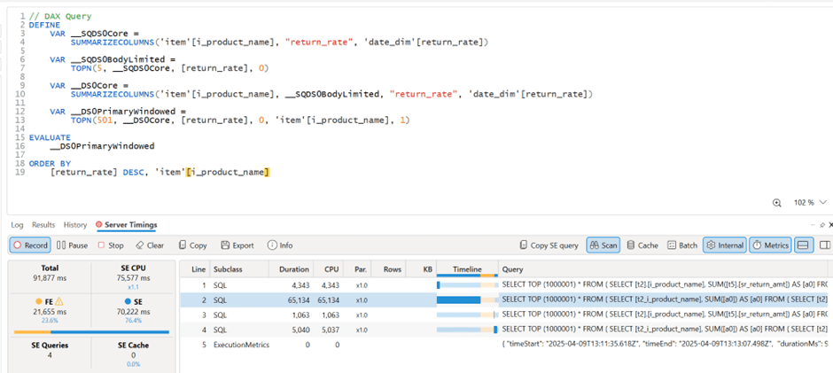
Power BI automatically generate SQL Queries based on the Data Model, Basically you defined measures using DAX, you add a visual which generate a DAX query that got translated to SQL, based on some complex logic, it may or may not push just 1 query to the source system, anyway in this case, it did generated multiple SQL queries and stitched the result together.
🔍 Insight: Power BI worked exactly as designed:
It split measures into independent queries.
It grouped by product_name, because that was the visible field in my model.
And surprisingly, it was faster than running the same query directly in DuckDB CLI!
Here’s my screenshot showing Power BI results and DAX Studio:
🧩 Step 3: DuckDB CLI — Slow with Text Joins
Running the same query directly in DuckDB CLI was noticeably slower, 290 seconds !!!
⚙️ Step 4: Manual SQL Tuning — Surrogate Keys Win
To fix this, I rewrote the SQL manually:
Switched to item_sk, a surrogate integer key.
Delayed lookup of human-readable fields.
Here’s the optimized query:
WITH sales_by_product AS (
    SELECT
        ss.ss_item_sk AS item_sk,
        SUM(ss.ss_sales_price * ss.ss_quantity) AS total_sales
    FROM store_sales ss
    GROUP BY ss.ss_item_sk
),

returns_by_product AS (
    SELECT
        sr.sr_item_sk AS item_sk,
        SUM(sr.sr_return_amt) AS total_returns
    FROM store_returns sr
    GROUP BY sr.sr_item_sk
),

combined AS (
    SELECT
        COALESCE(s.item_sk, r.item_sk) AS item_sk,
        COALESCE(s.total_sales, 0) AS total_sales,
        COALESCE(r.total_returns, 0) AS total_returns
    FROM sales_by_product s
    FULL OUTER JOIN returns_by_product r ON s.item_sk = r.item_sk
)

SELECT
    i.i_product_name AS product_name,
    ROUND((combined.total_returns / NULLIF(combined.total_sales, 0)) * 100, 2) AS return_rate
FROM combined
LEFT JOIN item i ON combined.item_sk = i.i_item_sk
WHERE i.i_product_name IS NOT NULL
ORDER BY return_rate DESC
LIMIT 5;
🚀 Result: Huge performance gain! from 290 seconds to 41 seconds
Check out the improved runtime in DuckDB CLI:
🌍 In real-world models, surrogate keys aren’t typically used
unfortunately in real life, people still use text as a join key, luckily PowerBI seems to do better there !!!
🚀 Final Thoughts
LLMs are funny, when I asked chatgpt why it did not suggest a better SQL Query, I got this answer 🙂
I guess the takeaway is this:
If you’re writing SQL queries, always prefer integer types for your keys!
And maybe, just maybe, DuckDB (and databases in general) could get even better at optimizing joins on text columns. 😉
But perhaps the most interesting question is: What if, one day, LLMs not only generate correct SQL queries but also fully performance-optimized ones?
Edit : run explain analyze show that it is group by is taking most of the time and not the joins
the optimized query assumed already that i.i_item_sk is unique, it is not very obvious for duckdb to rewrite the query without knowing the type of joins !!! I guess LLMs still have a lot to learn
DeltaProtocolError: The table has set these reader features: {'deletionVectors'} but these are not yet supported by the deltalake reader.
Alternative: Using DuckDB
A simple alternative is to use DuckDB:
import duckdb

duckdb.sql("SELECT COUNT(*) FROM delta_scan('/lakehouse/default/Tables/xxx')")
Tested with a file that contains Deletion vectors
Column Mapping
The same approach applies to column mapping as well.
Upgrading DuckDB
Currently, Fabric Notebook comes preinstalled with DuckDB version 1.1.3. To use the latest features, you need to upgrade to the latest stable release (1.2.1) :
Note: Installing packages using %pip install does not restart the kernel when you run the notebook , you need to use sys.exit(0) to apply the changes, as some packages may already be loaded into memory.
import duckdb
duckdb.sql(" force install delta from core_nightly ")
duckdb.sql(" from delta_scan('/lakehouse/default/Tables/dbo/evolution_column_change') ")
The Future of Delta Rust .
Currently, there are two Rust-based implementations of Delta:
Delta_rs: The first and more mature implementation, developed by the community. It is an independent implementation of the Delta protocol and utilizes DataFusion and PyArrow (which will soon be deprecated) as its engine. However, Delta_rs does not support deletion vectors or column mapping, though it does support writing Delta tables.
Delta Kernel_rs: The newer, “official” implementation of Delta, providing a low-level API for query engines. It is currently being adopted by DuckDB ( and Clickhouse apparently) with more engines likely to follow. However, it is still a work in progress and does not yet support writing.
There are ongoing efforts to merge Delta_rs with Delta Kernel_rs to streamline development and reduce duplication of work.
Note : although they are written in Rust, we mainly care about the Python API 🙂
Conclusion
At least for now, in my personal opinion, the best approach is to: