Category: parquet

TL:DR; Delta_rs does not support Vorder so we need workaround, we notice by changing row groups size and sorting data we improved a direct Lake model from not working at all to returning queries in 100 ms

I was having another look at Fabric F2 (hint: I like it very much; you can watch the video here). I tried to use Power BI in Direct Lake mode, but it did not work well, and I encountered memory errors. My first instinct was to switch it to Fabric DWH in Direct Query mode, and everything started working again.

Obviously, I did complain to the Power BI team that I was not happy with the results, and their answer was to just turn on V-order, which I was not using. I had used Delta_rs to write the Delta table, and the reason I never thought about Parquet optimization was that when I used F64, everything worked just fine since that SKU has more hardware. However, F2 is limited to 3 GB of RAM.

There are many scenarios where Fabric is primarily used for reading data that is produced externally. In such cases, it is important to understand how to optimize those Parquet files for better performance.

Phil Seamark (yes the same guy who built a 3D games using DAX) gave me some very good advice: you can still achieve very good performance even without using V-order. Just sort by date and partition as a first step, and you can go further by splitting columns.

As I got the report working perfectly, even inside F2, I thought it was worth sharing what I learned.

Note: I used the term ‘parquet’ as it is more relevant than specifying the table format, whether it is a Delta table or Iceberg, after all this is where the data is stored, there is no standard for Parquet layout, different Engines will produce different files with massive difference in row group, file size, encoding etc.

Memory Errors

This is not really something you would like to see, but that’s life. F2 is the lowest tier of Fabric, and you will encounter hardware limitations.

When trying to run a query from DAX Studio, you will get the same error:

Rule of Thumb

Split datetime into date and time

It may be a good idea to split the datetime column into two separate columns, date and time. Using a datetime column in a relationship will not give you good performance as it usually has a very high number of distinct values.

Reduce Precision if You Don’t Need It

If you have a number with a lot of decimals, changing the type to decimal(18,4) may give you better compression.

Sorting Data

Find Column Cardinality

First, let’s check the cardinality of all columns in the Delta table. I used DuckDB for this, but you can use any tool—it’s just a personal choice.

First, upgrade DuckDB and configure authentication:

!pip install -q duckdb --upgrade

token = notebookutils.credentials.getToken('storage')

duckdb.sql(f"""  
  CREATE OR REPLACE SECRET onelake (TYPE AZURE, PROVIDER ACCESS_TOKEN, ACCESS_TOKEN '{notebookutils.credentials.getToken('storage')}')  
""")

Then, run SUMMARIZE:

display(duckdb.sql(f"""  
  SUMMARIZE (from delta_scan('abfss://python@onelake.dfs.fabric.microsoft.com/data.Lakehouse/Tables/aemo/summary'))  
""").df())

And here is the result:

Automatic Sorting from Low to High Cardinality

A very simple rule is to sort the columns from low to high cardinality , in this example : time, duid, date, price, mw.

Columns like cutoff don’t matter as they have only one value.

The result isn’t too bad—I went from 753 MB to 643 MB.

However, this assumes that the column has a uniform data distribution, which is rarely the case in real life. In more serious implementations, you need to account for data skewness.

Sort Based on Query Patterns

I built the report, so I know exactly the types of queries. The main columns used for aggregation and filters are date and duid, so that’s exactly what I’m going to use: sort by date, then duid, and then from low to high cardinality.

I think I just got lucky—the size is now 444 MB, which is even better than V-order. Again, this is not a general rule; it just happened that for my particular fact table, with that particular data distribution, this ordering gave me better results.

But more importantly, it’s not just about the Parquet size. Power BI in Direct Lake mode (and import mode) can keep only the columns used by the query into memory at the row group level. If I query only the year 2024, there is a good chance that only the row groups containing that data will be kept into memory. However, for this to work, the data must be sorted. If 2024 data is spread all over the place, there is no way to page out the less used row groups.

edit : to be very clear, Vertipaq needs to see all the data to build a global dictionary, so initially all columns needed for a query has to be fully loaded into Memory.

More Advanced Sorting Heuristics

These are more complex row-reordering algorithms. Instead of simply sorting by columns, they analyze the entire dataset and reorder rows to achieve the best Run-Length Encoding (RLE) compression across all columns simultaneously. I suspect that V-order uses something similar, but this is a more complex topic that I don’t have much to say about.

To make matters more complex, it’s not just about finding a near-optimal solution; the algorithm must also be efficient. Consuming excessive computational resources to determine the best reordering might not be a practical approach.

If you are into this kind of thing, there is a nice phd thesis here to read

Split Decimal Numbers

Reducing column cardinality by splitting decimals into separate columns can also help. For example, instead of storing price = 73.3968, store it in two columns: 73 and 3968.

Indeed, this gave even better results—a size reduction to 365 MB.

To be totally honest, though, while it gave the best compression result, I don’t feel comfortable using it. Let’s just say it’s for aesthetic reasons, and because the data is used not only for Power BI but also for other Fabric engines. Additionally, you pay a cost later when combining those two columns.

Partitioning

Once the sorting is optimized, note that compression occurs at the row group level. Small row groups won’t yield better results.

For this particular example, Delta_rs generates row groups with 2 million rows, even when I changed the options. I might have been doing something wrong. Using Rust as an engine reduced it to 1 million rows. If you’re using Delta_rs, consider using pyarrow instead:

RG = 8_000_000

write_deltalake(
    path, df, mode="overwrite", 
    max_rows_per_file=RG, max_rows_per_group=RG, min_rows_per_group=RG, 
    engine="pyarrow"
)

Notice here, I’m not partitioning by column but by file. This ensures uniform row groups, even when data distribution is skewed. For example, if the year 2020 has 30M rows and 2021 has 50M rows, partitioning by year would create two substantially different Parquet files.

Testing Again in Fabric F2

Using F2 capacity, let’s see how the new semantic models behave. Notice that the queries are generated from the Power BI report. I manually used the reports to observe capacity behavior.

Testing Using DAX Studio

To understand how each optimization works, I ran a sample query using DAX Studio. Please note, this is just one query and doesn’t represent the complexity of existing reports, as a single report generates multiple queries using different group-by columns. So, this is not a scientific benchmark—just a rough indicator.

Make sure that PowerBI has no data in memory, you can use the excellent semantic lab for that

!pip install -q semantic-link-labs
import sempy_labs as labs
import sempy.fabric as fabric
def clear(sm):
    labs.refresh_semantic_model(sm, refresh_type='clearValues')
    labs.refresh_semantic_model(sm)
    return "done"
for x in ['sort_partition_split_columns','vorder','sort_partition','no_sort']:
    clear(x)

Cold Run

The cold run is the most expensive query, as VertiPaq loads data from OneLake and builds dictionaries in memory. Only the columns needed are loaded. Pay attention to CPU duration, as it’s a good indicator of capacity unit usage.

Warm Run

All queries read from memory, so they’re very fast, often completing in under 100 milliseconds, SQL endpoint return the data around 2 seconds, yes, it is way slower than vertipaq but virtually it does not consume any interactive compute.

using DAX Studio you can view the column loaded into Memory, any column not needed will not be loaded

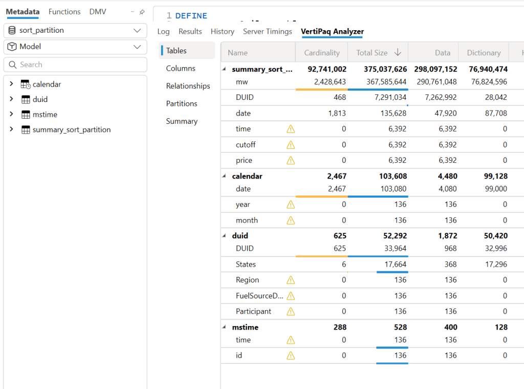
and the total data size into Memory

Hot Run

This isn’t a result cache. VertiPaq keeps the result of data scans in a buffer (possibly called datacache). If you run another query that can reuse the same data cache, it will skip an unnecessary scan. Fabric DWH would greatly benefit from having some sort of result cache (and yes, it’s coming).

Takeaways

• VertiPaq works well with sorted Parquet files. V-order is one way to achieve that goal, but it is not a strict requirement.
• RLE Encoding is more effective with larger row groups, and when the data is sorted
• Writing data in Fabric is inexpensive; optimizing for user-facing queries is more important.
• Don’t dismiss Direct Query mode in Fabric DWH—it’s becoming good enough for interactive, user-facing queries.
• Fabric DWH background consumption of compute unit is an attractive proposition
• Power BI will often read Parquet files written by Engines other than Fabric. A simple UI to display whether a Delta Table is optimized would be beneficial.
• Fabric DWH appears to handle less optimized Parquet files with greater tolerance