Getting different parties in the software industry to agree on a common standard is rare. Most of the time, a dominant player sets the rules. Occasionally, however, collaboration happens organically and multiple teams align on a shared approach. Geometry types in Parquet are a good example of that.
In short: there is now a defined way to store GIS data in Parquet. Both Delta Lake and Apache Iceberg have adopted the standard ( at least the spec). The challenge is that actual implementation across engines and libraries is uneven.
Iceberg: no geometry support yet in Java nor Python, see spec
Delta: it’s unclear if it’s supported in the open source implementation (I need to try sedona and report back), nothing in the spec though ?
DuckDB: recently added support ( you need nightly build or wait for 1.4)
PyArrow: has included support for a few months, just use the latest release
Arrow rust : no support, it means, no delta python support 😦
The important point is that agreeing on a specification does not guarantee broad implementation. and even if there is a standard spec, that does not means the initial implementation will be open source, it is hard to believe we still have this situation in 2025 !!!
Let’s run it in Python Notebook
To test things out, I built a Python notebook that downloads public geospatial data, merges it with population data, writes it to Parquet, and renders a map using GeoPandas, male sure to install the latest version of duckdb, pyarrow and geopandas
At first glance, that may not seem groundbreaking. After all, the same visualization could be done with GeoJSON. The real advantage comes from how geometry types in Parquet store bounding box coordinates. With this metadata, spatial filters can be applied directly during reads, avoiding the need to scan entire datasets.
That capability is what makes the feature truly valuable: efficient filtering and querying at scale, note that currently duckdb does not support pushing those filters, probably you need to wait to early 2026 ( it is hard to believe 2025 is nearly gone)
👉Workaround if your favorite Engine don’t support it .
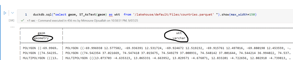
A practical workaround is to read the Parquet file with DuckDB (or any library that supports geometry types) and export the geometry column back as WKT text. This allows Fabric to handle the data, albeit without the benefits of native geometry support, For example PowerBI can read WKT just fine
duckdb.sql("select geom, ST_AsText(geom) as wkt from '/lakehouse/default/Files/countries.parquet' ")
For PowerBI support to wkt, I have written some blogs before, some people may argue that you need a specialized tool for Spatial, Personally I think BI tools are the natural place to display maps data 🙂
As a quick first impression, I tested Generating SQL Queries based on a YAML Based Semantic model, all the files are stored here , considering i have only 4 GB of VRAM, it is not bad at all !!!
to be clear, this is not a very rigorous benchmark, I just used the result of the last runs, differents runs will give you slightly different results, it is just to get a feeling about the Model, but it is a workload I do care about, which is the only thing that matter really.
The Experimental Setup
The experiment uses a SQL generation test based on the TPC-DS dataset (scale factor 0.1), featuring a star schema with two fact tables (store_sales, store_returns) and multiple dimension tables (date_dim, store, customer, item). The models were challenged with 20 questions ranging from simple aggregations to complex analytical queries requiring proper dimensional modeling techniques.
The Models Under Test
O3-Mini (Reference Model): Cloud-based Azure model serving as the “ground truth”
Qwen3-30B-A3B-2507: Local model via LM Studio
GPT-OSS-20B : Local model via LM Studio
Usually I use Ollama, but moved to LM studio because of MCP tools support, for Qwen 3, strangely code did not perform well at all, and the thinking mode is simply too slow
Key Technical Constraints
Memory Limit: Both local models run on 4GB VRAM, my laptop has 32 GB of RAM
Timeout: 180 seconds per query
Retry Logic: Up to 1 attempt for syntax error correction
Validation: Results compared using value-based matching (exact, superset, subset)
The Testing Framework
The experiment employs a robust testing framework with several features:
Semantic Model Enforcement
The models were provided with a detailed semantic model that explicitly defines:
Proper dimensional modeling principles
Forbidden patterns (direct fact-to-fact joins)
Required CTE patterns for combining fact tables
Specific measure definitions and business rules
Multi-Level Result Validation
Results are categorized into five match types:
Exact Match: Identical results including order
Superset: Model returns additional valid data
Subset: Model returns partial but correct data
Mismatch: Different results
Error: Execution or generation failures
The Results: Not bad at all
Overall Performance Summary
Both local models achieved 75-85% accuracy, which is remarkable considering they’re running on consumer-grade hardware with just 4GB VRAM. The GPT-OSS-20B model slightly outperformed Qwen3 with 85% accuracy versus 75%. Although it is way slower
I guess we are not there yet for interactive use case, it is simply too slow for a local setup, specially for complex queries.
Tool calling
a more practical use case is tools calling, you can basically use it to interact with a DB or PowerBI using an mcp server and because it is totally local, you can go forward and read the data and do whatever you want as it is total isolated to your own computer.
The Future is bright
I don’t want to sounds negative, just 6 months ago, i could not make it to works at all, and now I have the choice between multiple vendors and it is all open source, I am very confident that those Models will get even more efficient with time.
There are moments in life when you know things will never be the same. I remember distinctly when Gary showed me PowerPivot 10 years ago, and I knew that working with data would become as easy as playing with Excel. Another such moment was two days ago when I connected Claude Desktop to a database and asked, “What do you think?”
It was a strange experience. It wasn’t your typical “chat with your data and give me a nice chart” interaction. It was more like talking to a human and asking them to create a report. The LLM started by listing all the tables, examining the data, and making sense of what the dataset was about. Somehow, it figured out that the power generation figures were in MW and that to convert them to MWh, you need to divide by 12.
There’s a simple reason why this approach is so powerful compared to a typical chat with your data workflow: the LLM has read access to the data. It’s still secure and can only read what you’re authorized to access. As far as I know, these LLMs don’t auto-learn and don’t use the data for training, at least when you use an enterprise API.
Another interesting observation: as a non-programmer, I watched AI’s progress in coding with great excitement and never felt much sympathy for human coders. I thought they were exaggerating the threat. Somehow, my reaction changed when I noticed that AI will get very good at analytics too.
Note: I’ll refer to LLMs as AI for simplicity. Kurt has an excellent blog post worth reading, and thanks to Pawel for telling me about this whole MCP thing.
Typical “Chat with Your Data” Workflow
The important thing here is that AI doesn’t have access to your data at all. You collect the maximum knowledge about your data and send your questions with that knowledge. You get back SQL or DAX statements that you send to your server to get answers. if the question is not clear enough then they will ask for clarification, for example, what is the biggest country in the world, AI will reply, is it per size, by GDP etc, It’s much more complex in real life, but that’s the core idea.
Basically, we spend a lot of effort making sure AI can’t see your data. Sometimes, as a user, you wonder why this AI can’t answer some very obvious questions. Just imagine: as a data analyst, if someone asked you to give them a report without even seeing any numbers!
Using MCP
In this setup, the AI is unleashed. It can read the data directly (again, using only what you’re allowed to access and ideally read only), basically AI acts like an agent and has more autonomy, it is not limited only to your metadata.
Example Using Data from OneLake
I have this data in OneLake, and it’s cleansed data:
Because we don’t have an MCP server yet for Fabric DWH, I used the DuckDB MCP server to read the data from OneLake. For convenience, instead of using direct query, I imported the data into a local DuckDB file:
import duckdb

con = duckdb.connect()
con.sql("ATTACH 'aemo_delta.duckdb' AS db; USE db")

for tbl in ['duid', 'summary', 'calendar', 'mstdatetime']:
    con.sql(f"""
        CREATE OR REPLACE TABLE {tbl} AS
        FROM delta_scan('abfss://serving@onelake.dfs.fabric.microsoft.com/datamart.Lakehouse/Tables/aemo/{tbl}')
    """)

con.close()
You need to install MCP and configure the connection with Claude Desktop. To be clear, it should work with any MCP client, but so far, that’s the best I could find. Who knows, maybe one day Power BI Desktop will act as an MCP client (I literally made up this idea; this is not a hint or anything).
For me, it feels like ODBC for AI. The protocol is getting adopted by everyone.
The Experience
Since the data is public, I shared the whole chat. What I really like is how AI approaches the problem, first by looking at the tables. This is very human-like behavior.
If you read the chat, you’ll see it’s not perfect. It casually skipped hydro from the renewable conversation and didn’t calculate MWh correctly, although it did yesterday.
Some Observations
Even for a simple use case, you still need a semantic model. If I had a measure MWh = MW/12, the AI would always use it, at least in theory. For a complex model, it’s even more critical, Having said that, AI can do modeling just fine 🙂 do we need human for that ?
surprisingly in that simple workflow, i can replace every compute , what’s really critical is storage !!!
All my data is publicly available, so I wasn’t worried about security. For any enterprise work, you can’t really use something like Claude Desktop, but rather solutions like Azure AI Foundry.
For now, most models don’t acquire new knowledge during serving, but who knows what will happen in the next 10 years? You can imagine an AI that learns just from interaction with users and data, which opens all kinds of new questions. Do you need specific models for every tenant, for every user ? We’re not there yet, it is something we will have to deal with it.
I was giving a presentation about Microsoft Fabric Python notebooks and someone asked if they scale. The short answer is yes. You can download the notebook and try it for yourself. For the long answer, keep reading.
The dataset I used contains the last seven years of Australian electricity market data. Although it’s public, the government agency only keeps archives for two months. I had saved the data during a previous job and kept it around as a hobby. It’s a great real-world workload with realistic data distribution. The CSV files are messy. Technically, they’re more like reports, with different sections stacked on top of each other and varying numbers of columns. That’s often what you encounter in real projects, not the neat, well-structured datasets you see in demos.
For example, being able to read a CSV file with a variable number of columns is a critical feature. Yet this rarely gets mentioned in synthetic benchmarks.
To create a clean environment for testing, I copied the data from one Lakehouse in onelake to a brand-new workspace. I could have used a shortcut, but I wanted to start from scratch. The binary copy took just 2 minutes, with no transformations, which gives a throughput of 1.4 GB per second. That’s pretty good for a 150 GB uncompressed dataset.
The default configuration for Fabric Python notebooks includes 2 cores and 16 GB of RAM. That’s roughly the same size as Google Colab. But you can easily increase the number of cores to 4, 8, 16, 32, or even 64. At 64 cores, you get nearly half a terabyte of RAM. That’s a serious machine.
The job itself is simple. Ingest and process the data using several Python engines, then save the result as a Delta table. The raw data has around one billion records, and you end up extracting 311 million. If your engine cannot push down filters to the CSV level, you’re going to have a hard time. The trick here is not to be fast, but to avoid doing unnecessary work.
I used the following engines: DuckDB, Daft, Polars, CHDB (basically ClickHouse for Python), DataFusion, PyArrow, and Pandas. Technically, Pandas is not ideal here because you can’t pass a list of files without using a loop. But I had used it for nearly seven years, so I kept it for sentimental reasons.
I’m fairly confident using all of these engines except PyArrow and DataFusion. Their syntax is very intimidating, and I probably missed some configuration settings. I couldn’t get them to use more than a single thread, so CPU utilization stayed very low.
Results
Polars support streaming writes, but doesn’t allow exporting a record batch. This means the Delta writer has to load all data into memory. It works fine with 32 cores and 256 GB of RAM, but you’ll run into out-of-memory issues with 16 cores and below.
Chdb 3.5 added a user friendly way to export arrow record batch, it is the first release so still some bugs, for example got an error with 2 cores, I am sure it will get fixed soon
Daft is the only engine that supports native writing to Delta. It uses the Deltalake package only to commit the transaction log. The actual Parquet write is handled by the engine itself.
DuckDB preserves the sort order of the input files. it is trick to appeal to Pandas users who care about index ordering. For best performance though, you should turn this off. (Honestly, I think it should be off by default)
DuckDB exports Arrow tables by default. You need to explicitly use record_batch(). I’ve lost count of how many out-of-memory issues I’ve solved just by changing the export format.
Overall, DuckDB delivered the best performance, especially considering it’s not even writing Parquet files directly. It simply streams Arrow data to the writer.
When I first ran the test with DuckDB and saw it finish in under 4 minutes, I thought I made a mistake. It wasn’t until CHDB finished in under 5 minutes that I realized these engines are seriously impressive.
We’re talking about 625 MB per second for processing and ingestion on a single node.
Another key observation: using DuckDB and Daft, even with just 16 GB of RAM, the data was processed correctly. It took about an hour, but it worked without errors, that’s 10 X the size of the RAM
To verify correctness, I simply checked the total sum of a column and the number of records. Everything checked out.
Choosing the Right Size
Now that I know these notebooks work, choosing the right size becomes more nuanced. Surprisingly, the cheapest configuration in term of capacity usage was the 2 cores 🙂
In practice though, using more compute makes sense. A single node has no concept of fault tolerance. If something goes wrong, you need to restart the entire job. Personally, I’m not a fan of long-running jobs. Too many things can go wrong. I used 2 cores just to make a point. That said, using 64 cores doesn’t make much sense either. You’re doubling your compute cost to save 30 seconds.
One more thing: while Daft scales down very well, it doesn’t seem to scale up as efficiently as I had hoped. Ideally, you want a flat performance curve. The total amount of work is fixed, so adding more cores should just reduce execution time. I know the reality is more complex. It’s not easy to keep all processors busy at higher scales.
What This Means
As you may have guessed, I’m a big fan of single-node setups and DuckDB. But I don’t want just one engine to dominate every benchmark or deliver results that no other engine in its class can match. That’s why I was genuinely excited by Daft’s performance. I’m also looking forward to seeing Polars and CHDB add Arrow streaming support.
To be honest, I look at the world from a storage perspective. More competition between engines is a good thing. All of these tools are open source under the MIT license. Most of them can write to Delta in one form or another. and as a user you can choose any engine you want, I think that’s a fantastic thing to have.
So yes, Python notebooks do scale. The experience is far from being perfect, and there’s still room for improvement. But scalability is not something you should worry about, unless of course you are really doing real big data, then you go distributed 🙂 DWH and Spark are robust options in Fabric.
Edit : tested with chdb 3.5 which has support for arrow streaming