TL;DR: Iceberg’s value is sociological, not technical. And if you care about lightweight, single-process engines like datafusion and duckdb, it’s probably your best shot at first-class lakehouse support with Wide interoperability.
The first real data engineering work I did was an ingestion pipeline built on pandas and Parquet with Hive-style partitioning — an environment where 512 MB of memory was a genuine architectural constraint, not a rounding error. That experience shaped how I think about data tooling: the engine matters, but so does the ability to swap it out. Engine independence is something I care about more than most people I know, which is probably why I find myself paying close attention to Iceberg. Not for the reasons most people cite, though. It’s not the spec. It’s where the engineering hours are landing.
Getting query engines and catalogs to talk to each other is genuinely hard work. Most of it is unglamorous: error envelope parsing, metadata round-tripping, commit response shapes, partition spec edge cases, auth token quirks between vendors. None of it ships a feature anyone demos. None of it makes a good blog post. It’s the maintenance work that quietly determines whether your stack actually functions.
This is the part that’s easy to miss. Standards don’t converge because the spec is good. They converge because enough people, at enough companies, decide to put sustained hours into the interop bugs — year after year, across release cycles, through personnel changes and shifting priorities.
Look at the Iceberg committer list: Netflix, Apple, Databricks, Snowflake, AWS, Dremio, Microsoft. No single employer controls what gets merged. The incentive to fix cross-vendor interoperability bugs is distributed across the committer base itself. The governance isn’t just a formality — it’s what makes it possible for engineers from genuinely different setups to find, reproduce, and fix the same bug together.
There is one specific layer worth watching: the Iceberg REST catalog specification. It has become the canonical standard for how engines and catalogs communicate. Adoption is real: Polaris, lakekeeper, Gravitino, and a growing list of vendor-managed catalogs implement it.
But adoption and interoperability are not the same thing.
In practice, vendors still interpret parts of the specification differently. Engines end up handling quirks like slightly different response shapes, undocumented authentication flows, or inconsistent error handling. The nearest analogy is ODBC — a real standard, widely implemented, and still years of painful work before the “connect to anything” promise actually held up in practice.
The Iceberg REST catalog ecosystem feels earlier in that curve. The gap between specification and implementation is exactly where a lot of the maintenance work is happening right now. And closing that gap is precisely the kind of work Iceberg’s governance model is designed to support, because the people hitting the bugs are often the same people with commit access to fix them.
This is where the stakes become concrete, especially for lightweight engines.
For cloud warehouses and large JVM-based systems, the maintenance burden is manageable. There are full-time teams paid to absorb it. For the newer generation of small, single-process engines, the situation is very different. These are compact teams building engines with a specific focus: query latency, memory efficiency, embedded analytics, local execution.
Every hour spent chasing interoperability edge cases is an hour not spent improving the engine itself.
Several of these engines already support Iceberg in some form. But broad, reliable lakehouse support depends on the ecosystem doing its part: stable specifications, faithful implementations, bugs surfaced and fixed upstream.
A well-maintained standard is not just a convenience for these projects. It’s what makes serious lakehouse support achievable without hollowing out the team building the engine.
There is also a broader cost to fragmentation that rarely gets discussed directly. Every hour the ecosystem spends maintaining incompatible metadata layers is an hour not spent making lakehouse systems actually better. That cost doesn’t show up clearly in any individual issue tracker, but it accumulates across the entire ecosystem.
That’s the real argument for Iceberg.
Not that it’s a particularly clever format. Formats are mostly boring by design.
The real advantage is that Iceberg has assembled the right kind of maintenance coalition: enough companies with genuinely different incentives, governance that distributes merge authority, and enough independent implementations that bugs surface from the edges instead of only the center.
Whether that coalition survives long term as the market consolidates is still an open question. But right now, Iceberg is the ecosystem where the boring interoperability work is most likely to get done by someone other than you.
And in infrastructure, that’s close to everything.
That’s also why this feels personal to me.
The 512 MB pipeline I started with wrote Parquet files and hoped for the best — no transactions, no snapshot isolation, just partitions and careful scheduling to avoid stepping on yourself.
What I actually wanted, and couldn’t realistically have at the time, was proper ACID semantics with snapshot isloation end to end from something small and cheap. A cloud function. A tiny process with almost no memory to spare.
Iceberg is the closest thing to a realistic path toward that today. Not because the specification is especially elegant, but because it’s where the maintenance work is happening.
And eventually, ecosystems catch up to where the maintenance happens.
Special thanks to Raki Rahman for a few conversations that genuinely reshaped how I think about this space.
Microsoft Fabric lets you dynamically configure the number of vCores for a Python notebook session at runtime — but only when the notebook is triggered from a pipeline. If you run it interactively, the parameter is simply ignored and the default kicks in.
This is genuinely useful: you can right-size compute on a job-by-job basis without maintaining separate notebooks. A heavy backfill pipeline can request 32 cores; a lightweight daily refresh can get by with 2.
How It Works
Place a %%configure magic cell at the very top of your notebook (before any other code runs):
%%configure
{
"vCores":
{
"parameterName": "pipelinecore",
"defaultValue": 2
}
}
The parameterName field ("pipelinecore" here) is the name of the parameter you’ll pass in from the pipeline’s Notebook activity. The defaultValue is the fallback used when no parameter is provided — or when you run the notebook interactively.
Fabric supports vCore counts of 4, 8, 16, 32, and 64. Memory is allocated automatically to match.
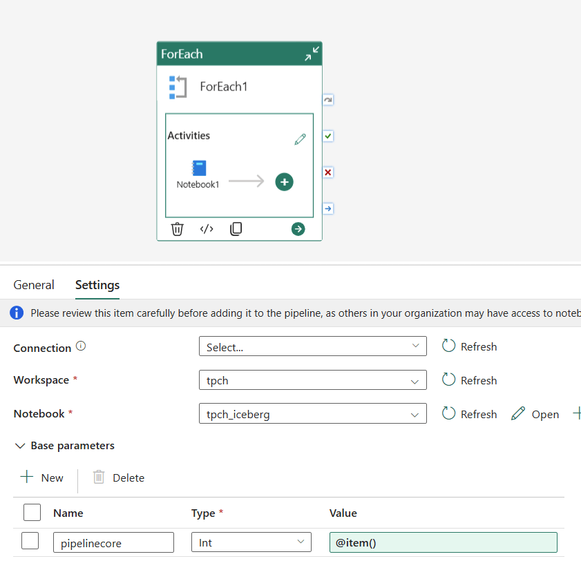
Wiring It Up in the Pipeline
In your pipeline, add a Notebook activity and open the Base parameters tab. Create a parameter named pipelinecore of type Int and set the value to @item().
When the pipeline runs, Fabric injects the value into %%configure before the session starts.
A Neat Trick: Finding the Right Compute Size
Because the vCore value is just a pipeline parameter, you can use a ForEach activity to run the same notebook across multiple core counts in sequence — great for benchmarking or profiling how your workload scales.
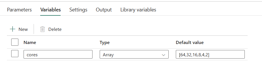
Set up a pipeline variable cores of type Array with a default value of [64,32,16,8,4,2]:
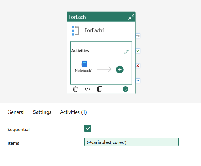
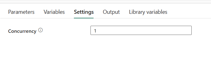
Then configure the ForEach activity with:
Items: @variables('cores')
Sequential: ✅ checked (so runs don’t overlap)
Concurrency: 1
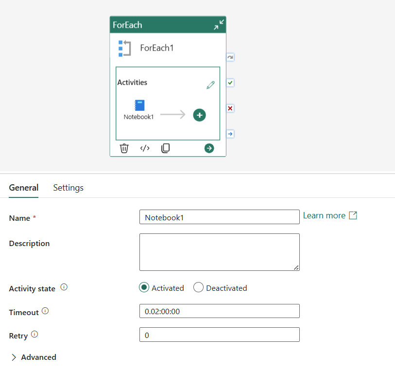
Inside the ForEach, add a Notebook activity and set the pipelinecore base parameter to @item(). Each iteration picks the next value from the array and passes it to the notebook, so you get a clean sequential run at 64, 32, 16, 8, 4, and 2 cores.
and of course the time, always change it to a more sensible value
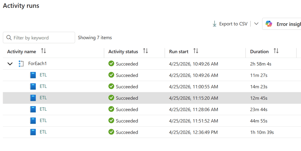
What the Numbers Say
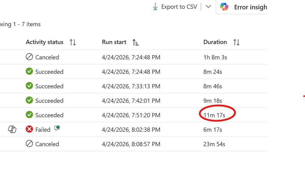
Running the previous workload across all supported core counts produced these results:
Cores
Duration
64
8m 24s
32
8m 46s
16
9m 18s
8
11m 17s
4
Failed
2
Canceled
The answer here is 8 cores. Yes, it’s about 2 minutes slower than 16 , but it’s half the compute. Going from 64 down to 8 cores costs you less than 3 minutes of runtime, which is a reasonable trade. Below 8 the workload simply falls apart. The sweet spot is not always the fastest run; it’s the point where adding more cores stops meaningfully improving the result.
btw for the CU consumption, the formula is very simple
nb of cores X 0.5 X active duration
Notice you will not be charged for startup duration.
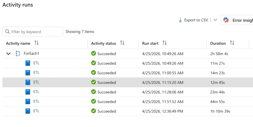
Another Workload: 158 GB of CSV with DuckDB
To make this concrete, here’s a second run — an ETL notebook processing 158 GB of CSV files using DuckDB 1.4.4, the default version available in the Fabric Python runtime.
I’d pick 16 cores here. The jump from 16 to 64 saves you barely a minute and a half — well within the noise, as 16 actually outran 32 in this test. Below 8 cores the runtime climbs steeply, roughly doubling at each step. The reason is that 158 GB of CSV is largely an I/O-bound workload: DuckDB parallelises reads aggressively, but at some point you’re just waiting on storage, not on CPU. More cores stop helping.
Two things worth noting. First, 2 cores completed the job — which is remarkable given that 2 cores comes with only 16 GB of RAM for a 158 GB dataset. DuckDB’s out-of-core execution handled it, but at 1h 10m it pushed close to the limit. And that brings up the second point: OneLake storage tokens have a lifetime of around one hour. A run that creeps past that boundary risks losing access mid-execution. For a workload this size, anything below 8 cores is probably not worth the gamble.
A Word of Caution: Startup Overhead
Before you start bumping up core counts, there’s an important trade-off to keep in mind: anything above 2 cores adds several minutes of python runtime just to provision the session — and that startup time is included in your total duration. For large, long-running workloads it barely registers. For small ones it can easily dominate the total run time.
And most real-world workloads are small. A daily incremental load, a lookup refresh, a small aggregation — these often complete in under a minute of actual computation. If the session startup costs you 3 minutes and the work itself costs 30 seconds, more cores aren’t helping.
The default of 2 cores starts fast and is the right choice for the majority of jobs. Reach for more only when you’ve measured that the workload actually benefits from it.
Beyond Benchmarking: Dynamic Resource Allocation
The benchmarking pattern is useful, but the more powerful idea is using this in production. Because the vCore count is just a number passed through the pipeline, nothing stops a first stage of your pipeline from deciding what that number should be.
Imagine a pipeline that starts by scanning a data lake to count the number of files or estimate the volume of data to process. Based on that output, it computes an appropriate core count and passes it to the notebook that does the actual work — 4 cores for a small daily increment, 32 for a full month’s backfill, 64 for a one-off historical load. The notebook itself doesn’t change; the compute scales to the workload automatically.
This kind of adaptive orchestration is normally something you’d build a lot of custom logic around. Here it’s just a parameter.
The Catch: Interactive Runs Use the Default
This only works end-to-end when triggered from a pipeline. Running the notebook manually in the Fabric UI will silently use the defaultValue — there’s no error, the parameter just won’t be overridden. Keep that in mind when testing.
TL;DR : The high-end version of this problem is mostly solved. GPT-4 or Claude Opus paired with a mature proprietary semantic layer like Microsoft Power BI’s will handle natural language queries reliably in production, This blog is a much narrower use case: how do small language models (4B parameters, 4GB VRAM) perform when paired with open-source semantic layers? not great, not terrible as of April 2026 😦
Running a 4B model through an immature open-source semantic layer on a laptop GPU is not a production architecture — but it turns out to be a surprisingly useful lens for measuring fundamental SLM progress. How much reasoning capability fits in 4GB? How well do small models follow explicit constraints? Where do they break down under complexity?
Curiosity is a valid reason to run a benchmark. even for fun
The hardware constraint is real. An NVIDIA RTX A2000 Laptop has 4GB VRAM. Models above ~4GB Q4_K_M overflow into Windows virtual memory and run painfully slow. The practical ceiling is a 4B parameter model at Q4_K_M quantization.
The bet: give a small model a semantic model as its system prompt, and it should close the gap. Encode the domain knowledge — measure definitions, join rules, anti-patterns — so the model doesn’t have to infer them from a raw schema. Reduce the cognitive load, reduce the capability requirements, get closer to fast and correct.
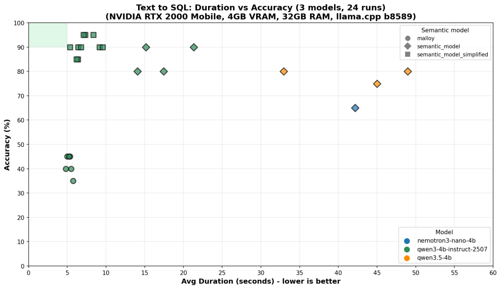
On the benchmark chart, that target lives in a small green rectangle in the top-left corner: high accuracy, low latency. This post is about what it takes to reach it — and why we’re still not reliably there.
What the Tests Measure
20 questions, graded from trivial to genuinely hard. Every answer is judged by exact result matching: every row must be correct, column order ignored, 0.5% numeric tolerance for floating point aggregations. Partial credit doesn’t exist.
The easy end (Q1–Q5): total revenue, total quantity sold, list of store names. Any model that can read a schema gets these right.
The hard end (Q18–Q20):
Return rate broken down by customer age group × weekend/weekday flag, joined through two fact tables
Brand-level year-over-year return rate change filtered by store state
Average net sales per transaction by item class and customer preferred flag
These require correctly combining multiple joins, conditional aggregations, and derived measures — and producing results that exactly match the reference answer.
Each run is plotted as accuracy vs. average duration per question. Speed matters because on 4GB VRAM, model size and inference cost are real constraints, not theoretical ones.
Results
One experiment: strip the full YAML semantic model (31KB, two explicit fact tables, extensive field metadata) down to a simplified version (23KB, single logical model, reduced noise). Less token budget spent on metadata, more focus on the patterns that matter.
Results across 3 models × 3 semantic model variants, 24 total runs:
                         Accuracy     Speed      Consistency
qwen3-4b + full model    ~90%         ~10s       scattered
qwen3-4b + simplified    ~90–95%      ~5–8s      tight → green box
nemotron + either        40–85%       ~5–12s     high variance regardless
qwen3.5-4b               ~75–80%      ~45–55s    slow regardless
A capable LLM writing raw SQL can score well on individual runs — 90%+ accuracy on the best models. That sounds promising until you look at the consistency column. The same question, asked twice, can produce correct SQL one run and wrong SQL the next. That variance doesn’t go away with better prompting — it’s a fundamental property of using a probabilistic model for a deterministic task.
Simplifying the semantic model helped the strongest model converge into the green box — higher accuracy, faster, more consistent. For weaker models, variance stayed high regardless of which semantic model they received. The bottleneck had shifted from context quality to model capability.
You cannot simplify your way past a capability ceiling.
Why Raw LLM Breaks
The failure patterns are specific and instructive.
The CTE + FULL OUTER JOIN pattern. The semantic model is explicit: never join the two fact tables (store_sales and store_returns) directly. Always aggregate each separately in a CTE, then combine with FULL OUTER JOIN. Direct joins cause row multiplication. When a model gets this wrong, the result looks plausible — same columns, similar numbers — but every figure is wrong. Models violate this more than you’d expect, especially when the question doesn’t obviously signal that two fact tables are involved.
-- Wrong: direct join multiplies rows
SELECT s.s_store_name, SUM(ss_sales_price * ss_quantity) as total_sales,
SUM(sr_return_amt) as total_returns
FROM store_sales ss
JOIN store_returns sr ON ss.ss_item_sk = sr.sr_item_sk
JOIN store s ON ss.ss_store_sk = s.s_store_sk
GROUP BY s.s_store_name;
-- Right: aggregate each fact separately, then join the summaries
WITH sales AS (
SELECT ss_store_sk, SUM(ss_sales_price * ss_quantity) as total_sales
FROM store_sales GROUP BY ss_store_sk
),
returns AS (
SELECT sr_store_sk, SUM(sr_return_amt) as total_returns
FROM store_returns GROUP BY sr_store_sk
)
SELECT s.s_store_name,
COALESCE(sales.total_sales, 0),
COALESCE(returns.total_returns, 0)
FROM store s
LEFT JOIN sales ON s.s_store_sk = sales.ss_store_sk
LEFT JOIN returns ON s.s_store_sk = returns.sr_store_sk;
Literal instructions ignored. Q9 requires the raw flag values as group labels: 'Y' and 'N', not 'Preferred' and 'Non-Preferred'. The semantic model says this explicitly. LLMs substitute human-readable labels anyway — not because they misread the instruction, but because “Preferred / Non-Preferred” is the more natural output. The model understood what you wrote. It decided it knew better.
These failures share a structure: the semantic model content is correct, but LLM use of it is unreliable. The context is a hint, not a guarantee. You cannot build a production analytics system on a component whose failure modes are unpredictable. Reliability requires a deterministic layer — a compiler that enforces the patterns, not a model that may or may not follow them.
The Right Architecture: LLM Intent + Deterministic Compilation
The right split between LLM and algorithm is this: use the LLM for what only an LLM can do, and use deterministic code for everything else.
Natural language understanding is irreducibly fuzzy — only the LLM can map “show me underperforming stores last quarter” to the right intent. But once that intent is expressed as a structured query, everything downstream is deterministic. The join logic, the measure definitions, the SQL generation — these are mechanical translations that a compiler does perfectly, every time, for free. Running them through an LLM instead wastes token budget on a task that doesn’t need intelligence, while leaving less capacity for the task that does.
The ideal split: the LLM translates natural language into a compact domain-specific query expression. The compiler translates that into SQL. The LLM never touches raw schema column names; the compiler never sees ambiguous natural language.
A query compiler is the right architecture for this problem. It’s deterministic: the same query gives the same answer every time. It enforces join logic and measure definitions by construction, not by suggestion. You can build systems around deterministic limitations. You cannot build systems around random failures.
The DSL the LLM targets doesn’t need to be as simple as SELECT measure FROM model GROUP BY dimension. Users ask for year-over-year comparisons, cohort breakdowns, conditional aggregations — the DSL has to be expressive enough to capture these. But “expressive enough for analytics” is still a far smaller language than SQL. The LLM has a much easier job expressing intent in a constrained, familiar DSL than generating arbitrarily complex raw SQL correctly every time.
Why Open-Source Compilers Aren’t There Yet
The current open-source implementations just aren’t there yet.
Fact-first structural limitations. Most open-source semantic layers are fact-first by design: all queries anchor to the fact table. “List all stores” should return 8 stores. Running through boring-semantic-layer, it returns 6 — stores with no sales are excluded because they have no fact rows. This is not an edge case; it breaks a whole category of queries that any real analytics system must handle. (see example here: boring-semantic-layer #224) Dimension-first routing — queries that go directly to dimension tables when no fact aggregation is needed — is a fundamental capability gap.
Niche query languages. Malloy compiles high-level queries to SQL — the LLM writes Malloy, the compiler handles join logic. In theory this is exactly right: offload SQL generation to a trusted compiler, let the LLM express what to compute. In practice, LLMs have seen enormous amounts of SQL during training and almost no Malloy. Syntax errors were common, measure references wrong. The compiler generated correct SQL from correct Malloy — but getting correct Malloy out of the LLM was harder than getting correct SQL directly.
The proprietary proof that this architecture is buildable: Microsoft Power BI’s query planner handles multi-fact joins, period-over-period comparisons, and dimension-first routing reliably, backed by years of engineering investment. The open-source ecosystem isn’t there yet — and there’s no guarantee it gets there. The commercial incentive that drove Power BI and Looker to solve these problems doesn’t exist for open-source projects in the same way.
The Ceiling Is Implementation Quality
The semantic model doesn’t need to pre-declare every possible query pattern — that’s the point of having an LLM in the loop. “Sales performance in 2020 vs 2021” should be composable: the SLM reads the base measures (total_sales, date_dim keys, grain definitions) and constructs the year-over-year logic itself. Multi-period comparisons, cohort filters, conditional aggregations — these should emerge from creative composition of well-defined primitives, not from an ever-growing library of pre-baked templates. The semantic model’s job is to define what things mean; the SLM’s job is to figure out how to combine them. When that division holds, the system is genuinely expressive. When it breaks down — when the SLM can’t compose reliably from primitives.
Query planner quality degrades fast once you move beyond simple aggregations. The moment you introduce measures that ignore filter context — MAX(date) computed across the full table regardless of what the user filtered — the planner has to reason about predicate pushdown, materialization order, and query cost. A naive planner gets this wrong silently: it scans everything, computes the max, then filters afterward. A recent semi-proprietary semantic layer ( which should remain nameless), supposedly mature, did exactly this on a simple max date ignore filter measure , a sub-second query became a 30-second full table scan.
Where This Goes
There are two truths that can coexist here.
On one side, models are clearly improving. Techniques like aggressive quantization are delivering more reasoning capability within tight resource constraints, making smaller deployments increasingly viable. At the same time, the architectural pattern of separating LLM intent from deterministic compilation is sound. It reflects how the most reliable production systems are built today. In that sense, the open source ecosystem is moving in the right direction, even if current implementations are still maturing.
On the other side, there is a meaningful gap between something being buildable and being built correctly. That gap is easy to underestimate. What looks like a working system often breaks down under real-world conditions: edge cases, ambiguous semantics, inconsistent schemas, and the need for cost-aware execution planning.
Bridging that gap is not just a matter of better ideas. It requires depth. Years of iteration, careful handling of corner cases, and continuous refinement of query planning and semantic layers. Systems like Power BI or Looker did not arrive there by accident. They reflect sustained, focused investment in exactly these problems.
Whether the open source ecosystem will reach that same level of depth remains an open question. It is not a question of capability or intent, but of coordination, time, and sustained effort across a fragmented landscape.
So the current state is this: the architecture is directionally correct, but the hardest parts are still unresolved, and progress on those parts is inherently slow.
Edit: There is also a credible alternative trajectory. If smaller language models continue to improve, direct SQL generation may become reliable enough for a large class of use cases. In that world, the need for a semantic query compiler does not disappear, but it becomes less central, reserved for cases where correctness, governance, or performance guarantees truly matter.
As a quick first impression, I tested Generating SQL Queries based on a YAML Based Semantic model, all the files are stored here , considering i have only 4 GB of VRAM, it is not bad at all !!!
to be clear, this is not a very rigorous benchmark, I just used the result of the last runs, differents runs will give you slightly different results, it is just to get a feeling about the Model, but it is a workload I do care about, which is the only thing that matter really.
The Experimental Setup
The experiment uses a SQL generation test based on the TPC-DS dataset (scale factor 0.1), featuring a star schema with two fact tables (store_sales, store_returns) and multiple dimension tables (date_dim, store, customer, item). The models were challenged with 20 questions ranging from simple aggregations to complex analytical queries requiring proper dimensional modeling techniques.
The Models Under Test
O3-Mini (Reference Model): Cloud-based Azure model serving as the “ground truth”
Qwen3-30B-A3B-2507: Local model via LM Studio
GPT-OSS-20B : Local model via LM Studio
Usually I use Ollama, but moved to LM studio because of MCP tools support, for Qwen 3, strangely code did not perform well at all, and the thinking mode is simply too slow
Key Technical Constraints
Memory Limit: Both local models run on 4GB VRAM, my laptop has 32 GB of RAM
Timeout: 180 seconds per query
Retry Logic: Up to 1 attempt for syntax error correction
Validation: Results compared using value-based matching (exact, superset, subset)
The Testing Framework
The experiment employs a robust testing framework with several features:
Semantic Model Enforcement
The models were provided with a detailed semantic model that explicitly defines:
Proper dimensional modeling principles
Forbidden patterns (direct fact-to-fact joins)
Required CTE patterns for combining fact tables
Specific measure definitions and business rules
Multi-Level Result Validation
Results are categorized into five match types:
Exact Match: Identical results including order
Superset: Model returns additional valid data
Subset: Model returns partial but correct data
Mismatch: Different results
Error: Execution or generation failures
The Results: Not bad at all
Overall Performance Summary
Both local models achieved 75-85% accuracy, which is remarkable considering they’re running on consumer-grade hardware with just 4GB VRAM. The GPT-OSS-20B model slightly outperformed Qwen3 with 85% accuracy versus 75%. Although it is way slower
I guess we are not there yet for interactive use case, it is simply too slow for a local setup, specially for complex queries.
Tool calling
a more practical use case is tools calling, you can basically use it to interact with a DB or PowerBI using an mcp server and because it is totally local, you can go forward and read the data and do whatever you want as it is total isolated to your own computer.
The Future is bright
I don’t want to sounds negative, just 6 months ago, i could not make it to works at all, and now I have the choice between multiple vendors and it is all open source, I am very confident that those Models will get even more efficient with time.