Experimenting with Text-to-SQL: Lessons from Optimizing Product Return Analysis

๐ŸŒŸ Introduction

While testing the DuckDB ODBC driver, which is getting better and better (not production ready but less broken compared to two years ago), I noticed something unexpected. Running queries through Power BI in DirectQuery mode was actually faster than executing them directly in the DuckDB native UI.

Naturally, that does not make sense !!!

What followed was an investigation that turned into a fun and insightful deep dive into text-to-SQL generation, Power BIโ€™s query behavior, and the enduring relevance of manual SQL tuning

๐Ÿงฉ The Goal: Find the Worst Product by Return Rate

The task was straightforward:

Calculate total sales, total returns, and return rate by product. Rank the products and find the top 5 with the highest return rates.

To make it interesting, I decided to try:

  1. Letting an LLM generate the SQL by loading the semantic model.
  2. Using PowerBI in Direct Query Mode.
  3. Finally, manually tuning the query.

๐Ÿ“ Step 1: LLM-generated SQL โ€” Clean and Understandable

chatgpt generated a good starting point:

WITH sales_by_product AS   (
SELECT
i.i_product_name AS product_name,
SUM(ss.ss_sales_price * ss.ss_quantity) AS total_sales
FROM store_sales ss
JOIN item i ON ss.ss_item_sk = i.i_item_sk
WHERE i.i_product_name IS NOT NULL
GROUP BY i.i_product_name
),

returns_by_product AS (
SELECT
i.i_product_name AS product_name,
SUM(sr.sr_return_amt) AS total_returns
FROM store_returns sr
JOIN item i ON sr.sr_item_sk = i.i_item_sk
WHERE i.i_product_name IS NOT NULL
GROUP BY i.i_product_name
),

combined AS (
SELECT
COALESCE(s.product_name, r.product_name) AS product_name,
COALESCE(s.total_sales, 0) AS total_sales,
COALESCE(r.total_returns, 0) AS total_returns
FROM sales_by_product s
FULL OUTER JOIN returns_by_product r
ON s.product_name = r.product_name
)

SELECT
product_name,
ROUND((total_returns / NULLIF(total_sales, 0)) * 100, 2) AS return_rate
FROM combined
WHERE total_sales > 0 -- Avoid divide by zero
ORDER BY return_rate DESC
limit 5 ;

โœ… Pros:

  • Clean and easy to read.
  • Logically sound.
  • Good for quick prototyping.

๐Ÿ” Observation: However, it used product_name (a text field) as the join key in the combined table, initially I was testing using TPC-DS10, the performance was good, but when I changed it to DS100, performance degraded very quickly!!! I should know better but did not notice that product_name has a lot of distinct values.

the sales table is nearly 300 M rows using my laptop, so it is not too bad

and it is nearly 26 GB of highly compressed data ( just to keep it in perspective)
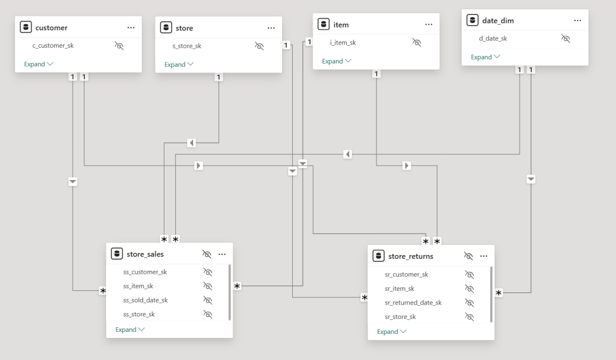
๐Ÿ“Š Step 2: Power BI DirectQuery Surprises

Power BI automatically generate SQL Queries based on the Data Model, Basically you defined measures using DAX, you add a visual which generate a DAX query that got translated to SQL, based on some complex logic, it may or may not push just 1 query to the source system, anyway in this case, it did generated multiple SQL queries and stitched the result together.

๐Ÿ” Insight: Power BI worked exactly as designed:

  • It split measures into independent queries.
  • It grouped by product_name, because that was the visible field in my model.
  • And surprisingly, it was faster than running the same query directly in DuckDB CLI!

Hereโ€™s my screenshot showing Power BI results and DAX Studio:
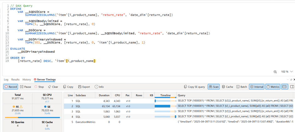

๐Ÿงฉ Step 3: DuckDB CLI โ€” Slow with Text Joins

Running the same query directly in DuckDB CLI was noticeably slower, 290 seconds !!!


โš™๏ธ Step 4: Manual SQL Tuning โ€” Surrogate Keys Win

To fix this, I rewrote the SQL manually:

  • Switched to item_sk, a surrogate integer key.
  • Delayed lookup of human-readable fields.

Hereโ€™s the optimized query:

WITH sales_by_product AS (
SELECT
ss.ss_item_sk AS item_sk,
SUM(ss.ss_sales_price * ss.ss_quantity) AS total_sales
FROM store_sales ss
GROUP BY ss.ss_item_sk
),

returns_by_product AS (
SELECT
sr.sr_item_sk AS item_sk,
SUM(sr.sr_return_amt) AS total_returns
FROM store_returns sr
GROUP BY sr.sr_item_sk
),

combined AS (
SELECT
COALESCE(s.item_sk, r.item_sk) AS item_sk,
COALESCE(s.total_sales, 0) AS total_sales,
COALESCE(r.total_returns, 0) AS total_returns
FROM sales_by_product s
FULL OUTER JOIN returns_by_product r ON s.item_sk = r.item_sk
)

SELECT
i.i_product_name AS product_name,
ROUND((combined.total_returns / NULLIF(combined.total_sales, 0)) * 100, 2) AS return_rate
FROM combined
LEFT JOIN item i ON combined.item_sk = i.i_item_sk
WHERE i.i_product_name IS NOT NULL
ORDER BY return_rate DESC
LIMIT 5;

๐Ÿš€ Result: Huge performance gain! from 290 seconds to 41 seconds

Check out the improved runtime in DuckDB CLI:


๐ŸŒ In real-world models, surrogate keys arenโ€™t typically used

unfortunately in real life, people still use text as a join key, luckily PowerBI seems to do better there !!!


๐Ÿš€ Final Thoughts

LLMs are funny, when I asked chatgpt why it did not suggest a better SQL Query, I got this answer ๐Ÿ™‚

I guess the takeaway is this:


If youโ€™re writing SQL queries, always prefer integer types for your keys!

And maybe, just maybe, DuckDB (and databases in general) could get even better at optimizing joins on text columns. ๐Ÿ˜‰

But perhaps the most interesting question is:
What if, one day, LLMs not only generate correct SQL queries but also fully performance-optimized ones?

Now that would be exciting.

you can download the data here, it is using very small factor : https://github.com/djouallah/Fabric_Notebooks_Demo/tree/main/SemanticModel

Edit : run explain analyze show that it is group by is taking most of the time and not the joins

the optimized query assumed already that i.i_item_sk is unique, it is not very obvious for duckdb to rewrite the query without knowing the type of joins !!! I guess LLMs still have a lot to learn

LLMs Are Getting Better at SQL

For no particular reason, I recently opened a Power BI report with two fact tables, exported the model definition to TMDL, saved it as a file, and loaded it into several state-of-the-art LLMs, including ChatGPT, Grok, Anthropic, and Qwen QWQ. I wasnโ€™t particularly interested in comparing specific modelsโ€”I just wanted to get a general sense of how they performed. To keep things simple, I used only the free tiers.

To my surprise, these models are getting really smart. They all recognized that the file represented a Power BI semantic model. They understood the concept of tables, columns, relationships, and measures, which was quite impressive.

You can download the Model here , i added a semantic Model as a text file in case you don’t have PowerBI

The Power of Semantic Models

Power BI, and before that PowerPivot, has supported multiple fact tables from day one. I remember the first time I used PowerPivotโ€” a colleague showed me how to handle multiple fact tables: just donโ€™t join fact to fact. Instead, use a common dimension, and everything will work fine. Back then, I had no idea about Kimball, multi-stage SQL queries, chasm trap etc. As a business user, I only cared that I got the correct results. It took me years to appreciate the ingenuity and engineering that went into making this work seamlessly. To me, this is an example of great product design: solve a very hard problem, and people will use it.

But this blog isnโ€™t about Power BI and DAXโ€”thatโ€™s a solved problem. Instead, I wanted to explore whether LLMs, by reading only metadata, could generate correct SQL queries for relatively complex questions.

Note: for people not familiar with TMDL, it is a human readable format of PowerBI semantic Model ( if human can read it, then LLMs will understand it too)

Testing LLMs with SQL Generation

I started with simple queries involving only one fact table, and the results were straightforward. The models correctly referenced measure definitions, avoiding column name hallucinations. Good news so far.

Things got more interesting when I asked for a query using a more complex measure, such as Net Sales:

Net Sales = [Total Sales] - [Total Returns]

This measure involves two tables: store_sales and store_returns.

Expected SQL Approach: Drilling Across

My expectation was that the models would use the Drilling Across technique. For example, when asked for net sales and cumulative sales by year and brand, a well-structured query would look like this:

  1. Compute total sales by year and brand.
  2. Compute total returns by year and brand.
  3. Join these results on year and brand.
  4. Calculate net sales as [Total Sales] - [Total Returns].
  5. Calculate cumulative Sales

Most LLMs generated a similar approach. Some required a hint (“donโ€™t ever join fact to fact”), but the biggest issue was the final join. Many models defaulted to a LEFT JOIN, which is problematicโ€”some returns for a brand might not occur in the same period as the sales, leading to incomplete results.

That said, some models got it right on the first attempt, which was very impressive. something like this:

WITH sales AS (
    SELECT
        d.d_year,
        i.i_brand,
        SUM(s.ss_sales_price * s.ss_quantity) AS total_sales
    FROM store_sales s
    JOIN item i ON s.ss_item_sk = i.i_item_sk
    JOIN date_dim d ON s.ss_sold_date_sk = d.d_date_sk
    GROUP BY d.d_year, i.i_brand
),
returns AS (
    SELECT
        d.d_year,
        i.i_brand,
        SUM(r.sr_return_amt) AS total_returns
    FROM store_returns r
    JOIN item i ON r.sr_item_sk = i.i_item_sk
    JOIN date_dim d ON r.sr_returned_date_sk = d.d_date_sk
    GROUP BY d.d_year, i.i_brand
)
SELECT
    COALESCE(s.d_year, r.d_year) AS year,
    COALESCE(s.i_brand, r.i_brand) AS brand,
    COALESCE(s.total_sales, 0) AS total_sales,
    COALESCE(r.total_returns, 0) AS total_returns,
    (COALESCE(s.total_sales, 0) - COALESCE(r.total_returns, 0)) AS net_sales,
    SUM(COALESCE(s.total_sales, 0) - COALESCE(r.total_returns, 0))
        OVER (PARTITION BY COALESCE(s.i_brand, r.i_brand) ORDER BY COALESCE(s.d_year, r.d_year)
        ROWS BETWEEN UNBOUNDED PRECEDING AND CURRENT ROW) AS cumulative_net_sales
FROM sales s
FULL OUTER JOIN returns r
ON s.d_year = r.d_year AND s.i_brand = r.i_brand
ORDER BY COALESCE(s.i_brand, r.i_brand), COALESCE(s.d_year, r.d_year);

An Alternative Approach: UNION ALL

One LLM got creative and proposed a different solution using UNION ALL:

WITH combined AS (
    SELECT d.d_year, i.i_brand, 'sales' AS type, s.ss_sales_price * s.ss_quantity AS amount
    FROM store_sales s
    JOIN date_dim d ON s.ss_sold_date_sk = d.d_date_sk
    JOIN item i ON s.ss_item_sk = i.i_item_sk
    UNION ALL
    SELECT d.d_year, i.i_brand, 'returns' AS type, r.sr_return_amt AS amount
    FROM store_returns r
    JOIN date_dim d ON r.sr_returned_date_sk = d.d_date_sk
    JOIN item i ON r.sr_item_sk = i.i_item_sk
)
SELECT
    d_year AS year,
    i_brand AS brand,
    SUM(CASE WHEN type = 'sales' THEN amount ELSE 0 END) AS total_sales,
    SUM(CASE WHEN type = 'returns' THEN amount ELSE 0 END) AS total_returns,
    (SUM(CASE WHEN type = 'sales' THEN amount ELSE 0 END) - SUM(CASE WHEN type = 'returns' THEN amount ELSE 0 END)) AS net_sales,
    SUM(SUM(CASE WHEN type = 'sales' THEN amount ELSE 0 END) - SUM(CASE WHEN type = 'returns' THEN amount ELSE 0 END))
        OVER (PARTITION BY i_brand ORDER BY d_year ROWS BETWEEN UNBOUNDED PRECEDING AND CURRENT ROW) AS cumulative_net_sales
FROM combined
GROUP BY d_year, i_brand
ORDER BY i_brand, d_year;

Edit : people who know what they are doing , did not like the union all solution for performance reason

So, Is SQL a Solved Problem?

No, of course not. Thereโ€™s still no guarantee of getting the same answer when asking the same question multiple times. Additionally, AI has no real understanding of the data. The moment you introduce filters, you can get all sorts of unexpected results,Although Providing sample values from columns into a semantic model helps a lot, still real-world models are far more complex and often contain ambiguities.

While LLMs generate correct SQL, they donโ€™t always generate the most efficient queries, But you can argue, it is the Database problem to solve ๐Ÿ™‚

Compute Considerations

I donโ€™t know enough to make a strong statement about the current cost of running LLMs, but I ran a simple experiment: I tested QWQ-32 on my laptop (which has an NVIDIA RTX A2000 GPU with 4GB of dedicated memory). The good news? It worked. Running an open-source “thinking model” on a personal laptop is already impressive. The bad news? It was painfully slowโ€”so much so that Iโ€™m not eager to repeat the test.

From a practical perspective, generating SQL queries this way seems extremely expensive. A decent BI tool can generate similar queries in milliseconds, using orders of magnitude less compute power, but as LLMs continue to improve in efficiency, maybe in a couple of years, the compute requirement to generate SQL Queries will become trivial ?

Final Thoughts

Having experimented with LLMs since 2023, I can say with confidence that they have improved significantly ( LLMs in 2023 were not very good to be honest). They are getting better and, more importantly, cheaper, opening the door for new applications.

The initial promise was that you could just throw data at an AI system, and it would figure out everything. I suspect thatโ€™s not true. In reality, to get useful results, you need more structure, and well-defined semantic models will play a crucial role in making asking your Data a reality.

Testing TPC-DS 10GB Hosted in Fabric OneLake Using Python Data Engines

This is not an official benchmarkโ€”just an exercise to experiment with the new Fabric Python notebook.

You can download the notebook and the results here

There is a growing belief that most structured data will eventually be stored in an open table format within object stores, with users leveraging various engines to query that data. The idea of data being tied to a specific data warehouse (DWH) may soon seem absurd, as everything becomes more open and interoperable.

While I canโ€™t predict the future, 2024 will likely be remembered as the year when the lakehouse concept decoupled from Spark. It has become increasingly common for “traditional” DWHs or any Database for that matter to support open table formats out of the box. Fabric DWH, for instance, uses a native storage layer based on Parquet and publishes Delta tables for consumption by other engines. Snowflake now supports Iceberg, and BigQuery is slowly adding support as well.

Iโ€™m not particularly worried about those DWH enginesโ€”they have thousands of engineers and ample resources, they will be doing just fine.

My interest lies more in the state of open source Python engines, such as Polars and DataFusion, and how they behave with a limited resource environment.

Benchmarking Bias

Any test inherently involves bias, whether conscious or unconscious. For interactive queries, SQL is the right choice for me. Iโ€™m aware of the various DataFrame APIs, but Iโ€™m not inclined to learn a new API solely for testing. For OLAP-type queries, TPC-DS and TPC-H are the two main benchmarks. This time, I chose TPC-DS for reasons explained later.

Benchmark Setup

All data is stored in OneLakeโ€™s Melbourne region, approximately 1,400 km away from my location, the code will check if the data exists otherwise it will be generated, the whole thing is fully reproducible.

I ran each query only once, ensuring that the DuckDB cache, which is temporary, was cleared between sessions. This ensures a fair comparison.

I explicitly used the smallest available hardware since larger setups could mask bottlenecks. Additionally, I have a specific interest in the Fabric F2 SKU.

While any Python library can be used, as of this writing, only two librariesโ€”DuckDB and DataFusionโ€”support:

  • Running the 99 TPC-DS queries (DataFusion supports 95, which is sufficient for me).
  • Native Delta reads for abfss or at least local paths.
  • Python APIs, as they are required to run queries in a notebook.

Other libraries like ClickHouse, Databend, Daft, and Polars lack either mature Delta support or compatibility with complex SQL benchmarks like TPC-DS.

Why TPC-DS ?

TPC-DS presents a significantly greater challenge than TPC-H, with 99 queries compared to TPC-Hโ€™s 22. Its more complex schema, featuring multiple fact and dimension tables, provides a richer and more demanding testing environment.

Why 10GB?

The 10GB dataset reflects the type of data I encountered as a Power BI developer. My focus is more on scaling down than scaling up. For context:

  • The largest table contains 133 million rows.
  • The largest table by size is 1.1GB.

Admittedly, TPC-DS 10GB is overkill since my daily workload was around 1GB. However, running it on 2 cores and 16GB of RAM highlights DuckDBโ€™s engineering capabilities.

btw, I did run the same test using 100GB and the python notebook with 16 GB did works just fine, but it took 45 minutes.

OneLake Access Modes

You can query OneLake using either abfss or mounted storage. I prefer the latter, as it simulates a local path and libraries donโ€™t require authentication or knowledge of abfss. Moreover, it caches data on runtime SSDs, which is an order of magnitude faster than reading from remote storage. Transactions are also included in the base capacity unit consumption, eliminating extra OneLake costs.

Itโ€™s worth noting that disk storage in Fabric notebook is volatile and only available during the session, while OneLake provides permanent storage.

You can read more about how to laverage DuckDB native storage format as a cache layer here

Onelake Open internet throughput

My internet connection is not too bad but not great either, I managed to get a peak of 113 Mbps, notice here the extra compute of my laptop will not help much as the bottleneck is network access.

Results

The table below summarizes the results across different modes, running both in Fabric notebooks and on my laptop.

  • DuckDB Disk caching yielded the shortest durations but the worst individual query performance, as copying large tables to disk takes time.
  • Delta_rs SQL performance was somewhat erratic.
  • Performance on my laptop was significantly slower, influenced by my internet connection speed.
  • Mounted storage offered the best overall experience, caching only the Parquet files needed for queries.

And here is the geomean

Key Takeaways

  • For optimal read performance, use mounted storage.
  • For write operations, use the abfss path.
  • Having a data center next to your laptop is probably a very good idea ๐Ÿ™‚

Due to network traffic, Querying inside the same region will be faster than Querying from the web (I know, it is a pretty obvious observation)

but is Onelake throughput good ?

I guess that’s the core question, to answer that I changed the Python notebook to use 8 cores, and run the test from my laptop using the same data stored in my SSD Disk, no call to onelake, and the results are just weird

Reading from Onelake using mounted storage in Fabric Notebook is faster than reading the same data from my Laptop !!!!

Looking Ahead to 2025

2024 has been an incredible year for Python engines, evolving from curiosities to tools supported by major vendors. However, as of today, no single Python library supports disk caching for remote storage queries. This remains a gap, and I hope itโ€™s addressed in 2025.

For Polars and Daft, seriously works on better SQL support

Optimizing Parquet Layout for Power BI Direct Lake Mode

TL:DR; Delta_rs does not support Vorder so we need workaround, we notice by changing row groups size and sorting data we improved a direct Lake model from not working at all to returning queries in 100 ms

I was having another look at Fabric F2 (hint: I like it very much; you can watch the video here). I tried to use Power BI in Direct Lake mode, but it did not work well, and I encountered memory errors. My first instinct was to switch it to Fabric DWH in Direct Query mode, and everything started working again.

Obviously, I did complain to the Power BI team that I was not happy with the results, and their answer was to just turn on V-order, which I was not using. I had used Delta_rs to write the Delta table, and the reason I never thought about Parquet optimization was that when I used F64, everything worked just fine since that SKU has more hardware. However, F2 is limited to 3 GB of RAM.

There are many scenarios where Fabric is primarily used for reading data that is produced externally. In such cases, it is important to understand how to optimize those Parquet files for better performance.

Phil Seamark (yes the same guy who built a 3D games using DAX) gave me some very good advice: you can still achieve very good performance even without using V-order. Just sort by date and partition as a first step, and you can go further by splitting columns.

As I got the report working perfectly, even inside F2, I thought it was worth sharing what I learned.

Note: I used the term ‘parquet’ as it is more relevant than specifying the table format, whether it is a Delta table or Iceberg, after all this is where the data is stored, there is no standard for Parquet layout, different Engines will produce different files with massive difference in row group, file size, encoding etc.

Memory Errors

This is not really something you would like to see, but thatโ€™s life. F2 is the lowest tier of Fabric, and you will encounter hardware limitations.

A screenshot of a computer

Description automatically generated

When trying to run a query from DAX Studio, you will get the same error:


Rule of Thumb

Split datetime into date and time

It may be a good idea to split the datetime column into two separate columns, date and time. Using a datetime column in a relationship will not give you good performance as it usually has a very high number of distinct values.

Reduce Precision if You Donโ€™t Need It

If you have a number with a lot of decimals, changing the type to decimal(18,4) may give you better compression.

Sorting Data

Find Column Cardinality

First, letโ€™s check the cardinality of all columns in the Delta table. I used DuckDB for this, but you can use any toolโ€”itโ€™s just a personal choice.

First, upgrade DuckDB and configure authentication:

!pip install -q duckdb --upgrade

token = notebookutils.credentials.getToken('storage')

duckdb.sql(f"""  
  CREATE OR REPLACE SECRET onelake (TYPE AZURE, PROVIDER ACCESS_TOKEN, ACCESS_TOKEN '{notebookutils.credentials.getToken('storage')}')  
""")

Then, run SUMMARIZE:

display(duckdb.sql(f"""  
  SUMMARIZE (from delta_scan('abfss://python@onelake.dfs.fabric.microsoft.com/data.Lakehouse/Tables/aemo/summary'))  
""").df())

And here is the result:

Automatic Sorting from Low to High Cardinality

A very simple rule is to sort the columns from low to high cardinality , in this example : time, duid, date, price, mw.

Columns like cutoff donโ€™t matter as they have only one value.

The result isnโ€™t too badโ€”I went from 753 MB to 643 MB.

However, this assumes that the column has a uniform data distribution, which is rarely the case in real life. In more serious implementations, you need to account for data skewness.


Sort Based on Query Patterns

I built the report, so I know exactly the types of queries. The main columns used for aggregation and filters are date and duid, so thatโ€™s exactly what Iโ€™m going to use: sort by date, then duid, and then from low to high cardinality.

I think I just got luckyโ€”the size is now 444 MB, which is even better than V-order. Again, this is not a general rule; it just happened that for my particular fact table, with that particular data distribution, this ordering gave me better results.

But more importantly, itโ€™s not just about the Parquet size. Power BI in Direct Lake mode (and import mode) can keep only the columns used by the query into memory at the row group level. If I query only the year 2024, there is a good chance that only the row groups containing that data will be kept into memory. However, for this to work, the data must be sorted. If 2024 data is spread all over the place, there is no way to page out the less used row groups.

edit : to be very clear, Vertipaq needs to see all the data to build a global dictionary, so initially all columns needed for a query has to be fully loaded into Memory.

More Advanced Sorting Heuristics

These are more complex row-reordering algorithms. Instead of simply sorting by columns, they analyze the entire dataset and reorder rows to achieve the best Run-Length Encoding (RLE) compression across all columns simultaneously. I suspect that V-order uses something similar, but this is a more complex topic that I donโ€™t have much to say about.

To make matters more complex, it’s not just about finding a near-optimal solution; the algorithm must also be efficient. Consuming excessive computational resources to determine the best reordering might not be a practical approach.

If you are into this kind of thing, there is a nice phd thesis here to read

Split Decimal Numbers

Reducing column cardinality by splitting decimals into separate columns can also help. For example, instead of storing price = 73.3968, store it in two columns: 73 and 3968.

Indeed, this gave even better resultsโ€”a size reduction to 365 MB.

To be totally honest, though, while it gave the best compression result, I donโ€™t feel comfortable using it. Letโ€™s just say itโ€™s for aesthetic reasons, and because the data is used not only for Power BI but also for other Fabric engines. Additionally, you pay a cost later when combining those two columns.

Partitioning

Once the sorting is optimized, note that compression occurs at the row group level. Small row groups wonโ€™t yield better results.

For this particular example, Delta_rs generates row groups with 2 million rows, even when I changed the options. I might have been doing something wrong. Using Rust as an engine reduced it to 1 million rows. If youโ€™re using Delta_rs, consider using pyarrow instead:

RG = 8_000_000

write_deltalake(
    path, df, mode="overwrite", 
    max_rows_per_file=RG, max_rows_per_group=RG, min_rows_per_group=RG, 
    engine="pyarrow"
)

Notice here, Iโ€™m not partitioning by column but by file. This ensures uniform row groups, even when data distribution is skewed. For example, if the year 2020 has 30M rows and 2021 has 50M rows, partitioning by year would create two substantially different Parquet files.

Testing Again in Fabric F2

Using F2 capacity, letโ€™s see how the new semantic models behave. Notice that the queries are generated from the Power BI report. I manually used the reports to observe capacity behavior.

A screenshot of a computer

Description automatically generated

Testing Using DAX Studio

To understand how each optimization works, I ran a sample query using DAX Studio. Please note, this is just one query and doesnโ€™t represent the complexity of existing reports, as a single report generates multiple queries using different group-by columns. So, this is not a scientific benchmarkโ€”just a rough indicator.

Make sure that PowerBI has no data in memory, you can use the excellent semantic lab for that

!pip install -q semantic-link-labs
import sempy_labs as labs
import sempy.fabric as fabric
def clear(sm):
    labs.refresh_semantic_model(sm, refresh_type='clearValues')
    labs.refresh_semantic_model(sm)
    return "done"
for x in ['sort_partition_split_columns','vorder','sort_partition','no_sort']:
    clear(x)

Cold Run

The cold run is the most expensive query, as VertiPaq loads data from OneLake and builds dictionaries in memory. Only the columns needed are loaded. Pay attention to CPU duration, as itโ€™s a good indicator of capacity unit usage.

Warm Run

All queries read from memory, so theyโ€™re very fast, often completing in under 100 milliseconds, SQL endpoint return the data around 2 seconds, yes, it is way slower than vertipaq but virtually it does not consume any interactive compute.

using DAX Studio you can view the column loaded into Memory, any column not needed will not be loaded

and the total data size into Memory

Hot Run

This isnโ€™t a result cache. VertiPaq keeps the result of data scans in a buffer (possibly called datacache). If you run another query that can reuse the same data cache, it will skip an unnecessary scan. Fabric DWH would greatly benefit from having some sort of result cache (and yes, itโ€™s coming).

Takeaways

  • VertiPaq works well with sorted Parquet files. V-order is one way to achieve that goal, but it is not a strict requirement.
  • RLE Encoding is more effective with larger row groups, and when the data is sorted
  • Writing data in Fabric is inexpensive; optimizing for user-facing queries is more important.
  • Donโ€™t dismiss Direct Query mode in Fabric DWHโ€”itโ€™s becoming good enough for interactive, user-facing queries.
  • Fabric DWH background consumption of compute unit is an attractive proposition
  • Power BI will often read Parquet files written by Engines other than Fabric. A simple UI to display whether a Delta Table is optimized would be beneficial.
  • Fabric DWH appears to handle less optimized Parquet files with greater tolerance