TL;DR: Incremental framing is like CDC to RAM 🙂 It significantly improves cold-run performance of Direct Lake mode in some scenarios, there is an excellent documentation that explain everything in details
What Is Incremental Framing?
One of the most important improvements to Direct Lake mode in Power BI is incremental framing.
Power BI’s OLAP engine, VertiPaq (probably the most widely deployed OLAP engine, though many outside the Power BI world may not know it) relies heavily on dictionaries. This works well because it is a read-only database. another core trick is its ability to do calculation directly on encoded data. This makes it extremely efficient and embarrassingly fast ( I just like this expression for some reason ).
Direct Lake Breakthrough
Direct Lake’s breakthrough is that dictionary building is fast enough to be done at runtime.
Typical workflow:
- A user opens a report.
- The report generates DAX queries.
- These queries trigger scans against the Delta table.
- VertiPaq scans only the required columns.
- It builds a global dictionary per column, loads the data from Parquet into memory, and executes queries.
The encoding step happens once at the start, and since BI data doesn’t usually change more that much, this model works well.
The Problem with Continuous Appends
In scenarios where data is appended frequently (e.g., every few minutes), the initial approach does not works very well. Each update requires rebuilding dictionaries and reloading all the data into RAM, effectively paying the cost of a cold run every time ( reading from remote storage will be always slower).
How Incremental Framing Fixes This
Incremental framing solves the problem by:
- Incrementally loading new data into RAM.
- Encoding only what’s necessary.
- Removing obsolete Parquet data when not needed.
This substantially improves cold-run performance. Hot-run performance remains largely unchanged.
Benchmark: Australian Electricity Market
To test this feature, I used my go-to workload: the Australian electricity market, where data is appended every 5 minutes—an ideal test case.
- Incremental framing is on by default, I turn it off using this bog
- For benchmarking, I adapted an existing tool , Direct Lake load testing( I just changed writing the results to Delta instead of CSV), I used 8 concurrent users, the main fact Table is around 120 M records, the queries reflect a typical user session , this is a real life use case, not some theoretical benchmark.
Results
P99
P99 (the 99th percentile latency, often used to show worst-case performance):
- Improvement of 9x–10x, again, your results may varied depending on workload, Parquet layout, and data distribution.

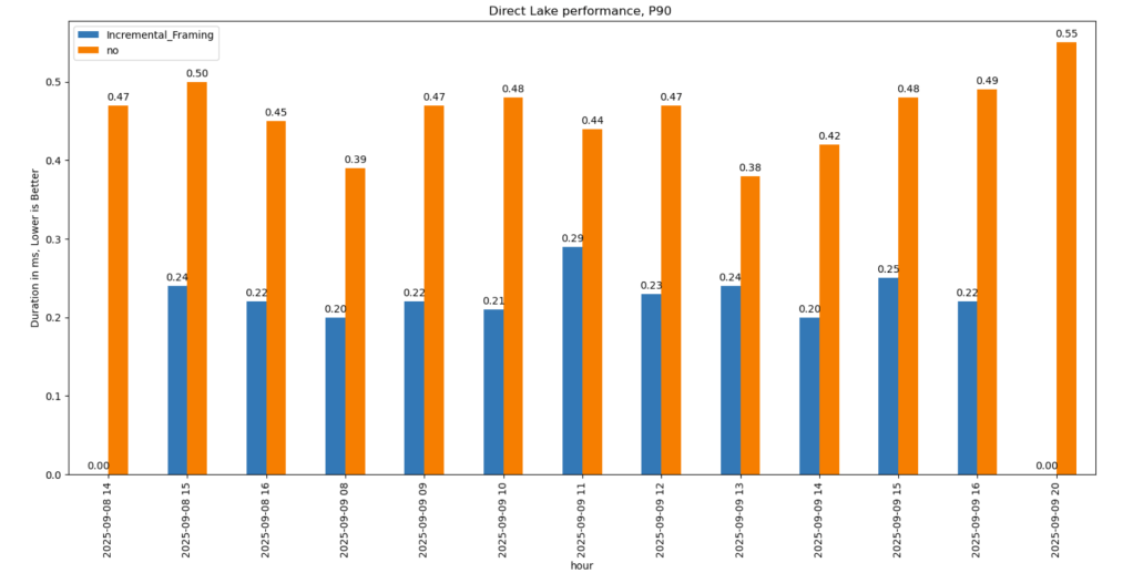
P90
P90 (90th percentile latency):
- Less dramatic but still strong.
- Improved from 500 ms → 200 ms.
- Faster queries also reduce capacity unit usage.
Geomean
just for fun and to show how fast Vertipaq is, let’s see the geomean, alright went from 11 ms to 8 ms, general purpose OLAP engines are cool, but specialized Engines are just at another level !!!

This does not solve Bad Table layout problem
This feature improves support for Delta tables with frequent appends and deletes. However, performance still degrades if you have too many small Parquet row groups.
VertiPaq does not rewrite data layouts—it reads data as-is. To maintain good performance:
- Compact your tables regularly.
- In my case, I backfill data nightly. The small Parquets added during the day don’t cause major issues, but I still compact every 100 files as a precaution.
If your data is produced inside Fabric, VOrder helps manage this. For external engines (Snowflake, Databricks, Delta Lake with Python), you’ll need to actively manage table layout yourself.