While preparing for a presentation about the FabCon announcement, one item was about OneLake Diagnostics. all ll I knew was that it had something to do with security and logs. As a Power BI user, that’s not exactly the kind of topic that gets me excited, but I needed to know at least the basic, so I can answer questions if someone ask 🙂
Luckily, we have a tradition at work , whenever something security-related comes up, we just ping Amnjeet 🙂
He showed me how it works , and I have to say, I loved it. It’s refreshingly simple.
You can download the notebook here:
You just select a folder in your Lakehouse and turn it on.

That’s it , the system automatically starts generating JSON files, neatly organized using Hive-style partitions, By default, user identity and IP tracking are turned off unless an admin explicitly enables them. You can find more details about the schema and setup here.
What the Logs Look Like

Currently, the logs are aggregated at the hourly level, but the folder structure also includes a partition for minutes (even though they’re all grouped at 00 right now).
Parsing the JSON Logs
Once the logs were available, I wanted to do some quick analysis , not necessarily about security, just exploring what’s inside.
There are probably half a dozen ways to do this in Fabric ; Shortcut Transform, RTI, Dataflow Gen2, DWH, Spark, and probably some AI tools too, Honestly, that’s a good problem to have.
But since I like Python notebooks and the data is relatively small, I went with DuckDB (as usual), but Instead of using plain DuckDB and delta_rs to store the results, I used my little helper library, duckrun, to make things simpler ( Self Promotion alert).
Then I asked Copilot to generate a bit of code for registering existing functions to look up the workspace name and lakehouse name from their GUIDs in DuckDB, using SQL to call python is cool 🙂
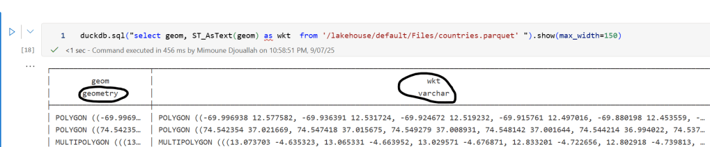
The data is stored incrementally, using the file path as a key , so you end up with something like this:
import duckrun

con = duckrun.connect('bigdata/tpch.lakehouse/dbo')

onelake_logs_path = (
    'abfss://bigdata@onelake.dfs.fabric.microsoft.com/'
    'tpch.Lakehouse/Files/DiagnosticLogs/OneLake/Workspaces/*/'
    'y=*/m=*/d=*/h=*/m=*/*.json'
)
Then I added only the new logs with this SQL script:
try:
    con.sql(f"""
        CREATE VIEW IF NOT EXISTS logs(file) AS SELECT 'dummy';
        SET VARIABLE list_of_files =
        (
            WITH new_files AS (
                SELECT file
                FROM glob('{onelake_logs_path}')
                WHERE file NOT IN (SELECT DISTINCT file FROM logs)
                ORDER BY file
            )
            SELECT list(file) FROM new_files
        );
        SELECT * EXCLUDE(data), data.*, filename AS file
        FROM read_json_auto(
            GETVARIABLE('list_of_files'),
            hive_partitioning = true,
            union_by_name = 1,
            FILENAME = 1
        )
    """).write.mode("append").option("mergeSchema", "true").saveAsTable('logs')
except Exception as e:
    print(f"An error occurred: {e}")
1- Using glob() to collect file names means you don’t open any files unnecessarily , a small but nice performance win.
2- DuckDB expand the struct using this expression data.*
3- union_by_name = 1 in case the json has different schemas
4- option(“mergeSchema”, “true”) for schema evolution in Delta table
Exploring the Data
Once the logs are in a Delta table, you can query them like any denormalize table.
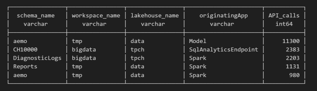
For example, here’s a simple query showing API calls per engine:
Note : using AI to get working regex is maybe the best thing ever 🙂
SELECT
    regexp_extract(resource, '([^&/]+)/([^&/]+)/(Tables|Files)(?:/([^&/]+))?(?:/([^&/]+))?', 4) AS schema_name,
    get_workspace_name(workspaceid) AS workspace_name,
    get_lakehouse_name(workspaceid, itemId) AS lakehouse_name,
    originatingApp,
    COUNT(*) AS API_calls
FROM logs
GROUP BY ALL
ORDER BY API_calls DESC
LIMIT 5;

Fun fact: OneLake tags Python notebook as Spark.
Also, I didn’t realize Lineage calls OneLake too!
as I have already register Python functions as UDFs, which is how I pulled in the workspace and lakehouse names in the query above.
Takeaway
This was just a bit of tinkering, but I’m really impressed with how easy OneLake Diagnostics is to set up and use.
I still remember the horrors of trying to connect Dataflow Gen1 to Azure Storage ,that was genuinely painful (and I never even got access from IT anyway).
It’s great to see how Microsoft Fabric is simplifying these scenarios. Not everything can always be easy, but making the first steps easy really gives the feature a very good impression.