just vorder don’t try to understand how vertipaq works

I know it is a niche topic, and in theory, we should not think about it. in import mode, Power BI ingests data and automatically optimizes the format without users knowing anything about it. With Direct Lake, it has become a little more nuanced. The ingestion part is done downstream by other processes that Power BI cannot control. The idea is that if your Parquet files are optimally written using Vorder, you will get the best performance. The reality is a bit more complicated. External writers know nothing about Vorder, and even some internal Fabric Engines do not write it by default.

To show the impact of read performance for Vordered Parquet vs sorted Parquet, I ran some tests. I spent a lot of time ensuring I was not hitting the hot cache, which would defeat the purpose. One thing I learned is to test only one aspect of the system carefully.

Cold Run: Data loaded from OneLake with on-the-fly building of dictionaries, relationships, etc

Warm Run: Data already in memory format.

Hot Run: The system has already scanned the same data before. You can disable this by calling the ClearCache command using XMLA (you cannot use a REST API call).
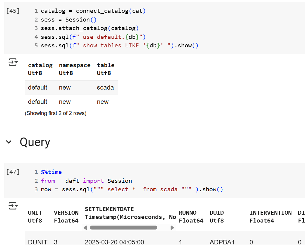

Prepare the Data

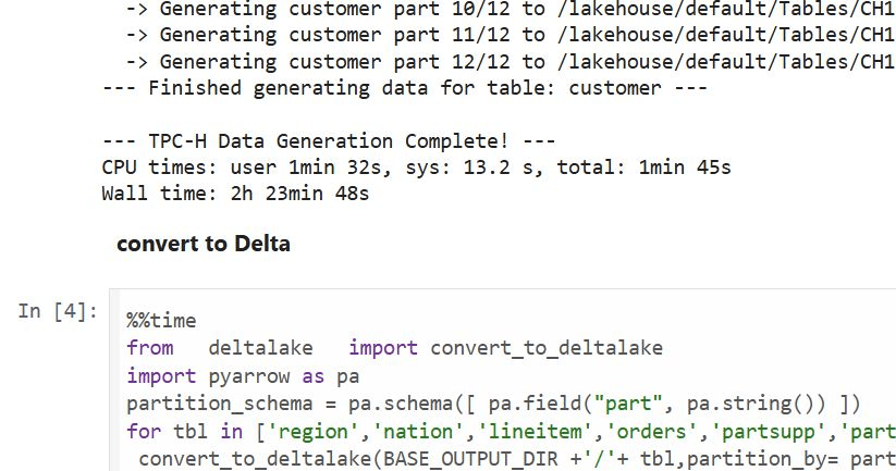
Same model, three dimensions, and one fact table, you can generate the data using this notebook

  • Deltars: Data prepared using Delta Rust sorted by date, id, then time.
  • Spark_default: Same sorted data but written by Spark.
  • Spark_vorder: Manually enabling Vorder (Vorder is off by default for new workspaces).

Note: you can not sort and vorder at the same time, at least in Spark, DWH seems to support it just fine

The data layout is as follows:

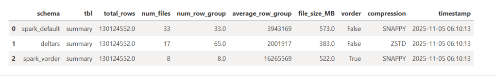
I could not make Delta Rust produce larger row groups. Notice that ZSTD gives better compression, although it seems Power BI has to uncompress the data in memory, so it seems it is not a big deal

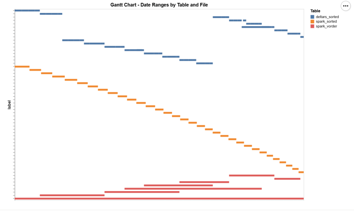
I added a bar chart to show how the data is sorted per date. As expected, Vorder is all over the place, the algorithm determines that this is the best row reordering to achieve the best RLE encoding.


The Queries

The queries are very simple. Initially, I tried more complex queries, but they involved other parts of the system and introduced more variables. I was mainly interested in testing the scan performance of VertiPaq.

Basically, it is a simple filter and aggregation.


The Test

You can download the notebook here :

def run_test(workspace, model_to_test):
    for i, dataset in enumerate(model_to_test):
        try:
            print(dataset)
            duckrun.connect(f"{ws}/{lh}.Lakehouse/{dataset}").deploy(bim_url)
            run_dax(workspace, dataset, 0, 1)
            time.sleep(300)
            run_dax(workspace, dataset, 1, 5)
            time.sleep(300)
        except Exception as e:
            print(f"Error: {e}")
    return 'done'

Deploy automatically generates a new semantic model. If it already exists, it will call clearvalue and perform a full refresh, ensuring no data is kept in memory. When running DAX, I make sure ClearCache is called.

The first run includes only one query; the second run includes five different queries. I added a 5-minute wait time to create a clearer chart of capacity usage.


Capacity Usage

To be clear, this is not a general statement, but at least in this particular case with this specific dataset, the biggest impact of Vorder seems to appear in the capacity consumption during the cold run. In other words:

Transcoding a vanilla Parquet file consumes more compute than a Vordered Parquet file.

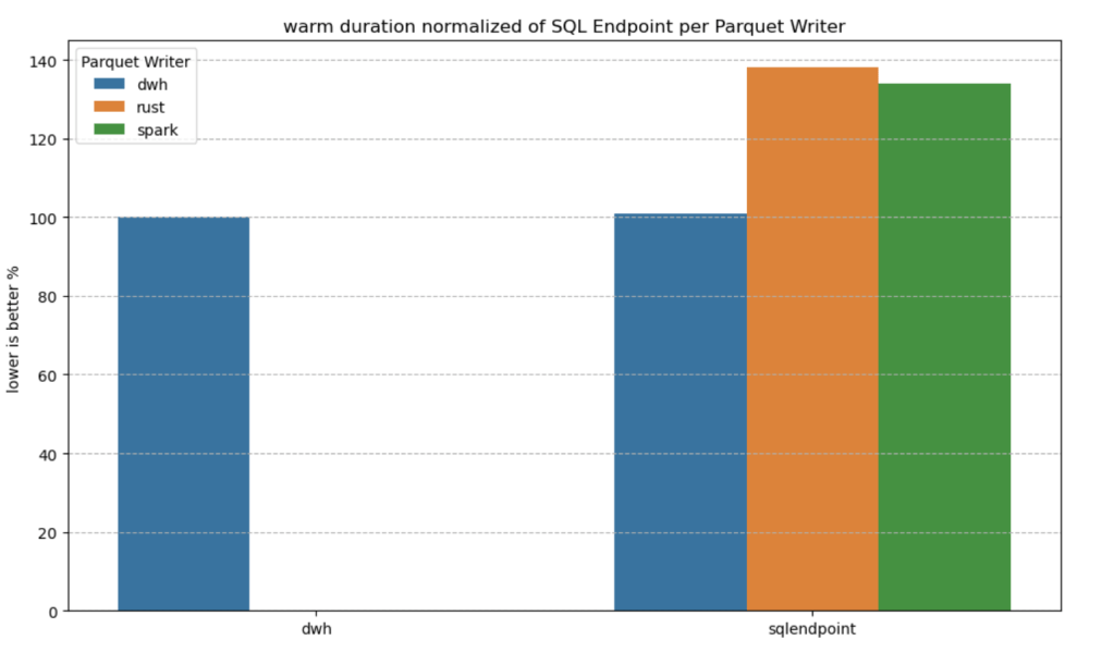
Warm runs appear to be roughly similar.


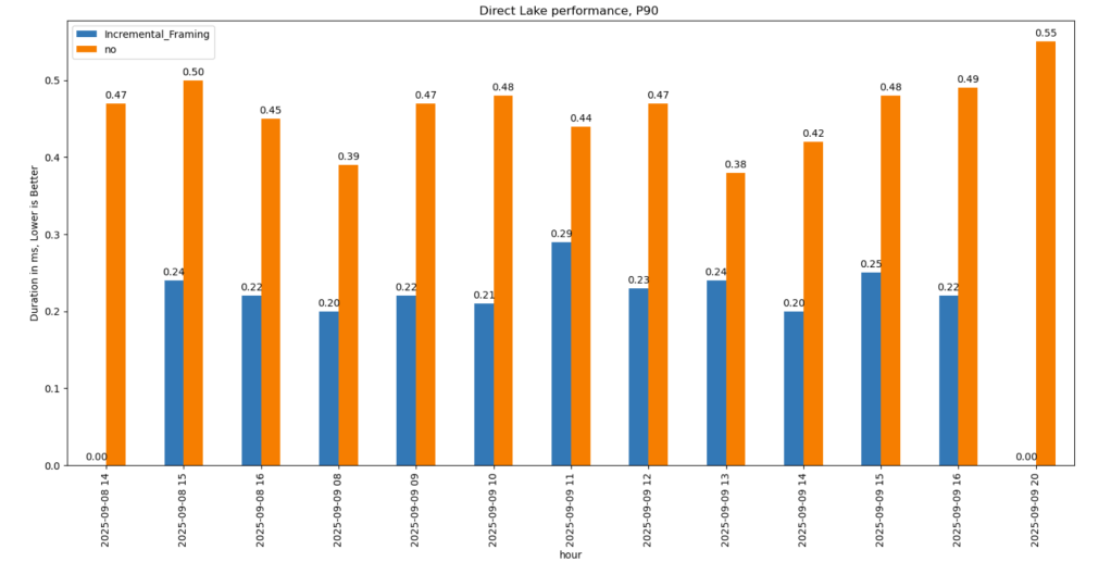
Impact on Performance

Again, this is based on only a couple of queries, but overall, the sorted data seems slightly faster in warm runs (although more expensive). Still, 120 ms vs 340 ms will not make a big difference. I suspect the queries I ran aligned more closely with the column sorting—that was not intentional.


Takeaway

Just Vorder if you can. Make sure you enable it when starting a new project. ETL, data engineering have only one purpose, make the experience of the end users the best possible way, ETL job that take 30 seconds more is nothing compared to a slower PowerBI reports.

now if you can’t, maybe you are using a shortcut from an external engine, check your powerbi performance if it is not as good as you expect then make a copy, the only thing that matter is the end user experience.

Another lesson is that VertiPaq is not your typical OLAP engine; common database tricks do not apply here. It is a unique engine that operates entirely on compressed data. Better-RLE encoded Parquet will give you better results, yes you may have cases where the sorting align better with your queries pattern, but in the general case, Vorder is always the simplest option.

First Look at Incremental Framing in Power BI

TL;DR: Incremental framing is like CDC to RAM 🙂 It significantly improves cold-run performance of Direct Lake mode in some scenarios, there is an excellent documentation that explain everything in details

What Is Incremental Framing?

One of the most important improvements to Direct Lake mode in Power BI is incremental framing.

Power BI’s OLAP engine, VertiPaq (probably the most widely deployed OLAP engine, though many outside the Power BI world may not know it) relies heavily on dictionaries. This works well because it is a read-only database. another core trick is its ability to do calculation directly on encoded data. This makes it extremely efficient and embarrassingly fast  ( I just like this expression for some reason ).


Direct Lake Breakthrough

Direct Lake’s breakthrough is that dictionary building is fast enough to be done at runtime.

Typical workflow:

  1. A user opens a report.
  2. The report generates DAX queries.
  3. These queries trigger scans against the Delta table.
  4. VertiPaq scans only the required columns.
  5. It builds a global dictionary per column, loads the data from Parquet into memory, and executes queries.

The encoding step happens once at the start, and since BI data doesn’t usually change more that much, this model works well.


The Problem with Continuous Appends

In scenarios where data is appended frequently (e.g., every few minutes), the initial approach does not works very well. Each update requires rebuilding dictionaries and reloading all the data into RAM, effectively paying the cost of a cold run every time ( reading from remote storage will be always slower).


How Incremental Framing Fixes This

Incremental framing solves the problem by:

  • Incrementally loading new data into RAM.
  • Encoding only what’s necessary.
  • Removing obsolete Parquet data when not needed.

This substantially improves cold-run performance. Hot-run performance remains largely unchanged.


Benchmark: Australian Electricity Market

To test this feature, I used my go-to workload: the Australian electricity market, where data is appended every 5 minutes—an ideal test case.

  • Incremental framing is on by default, I turn it off using this bog
  • For benchmarking, I adapted an existing tool , Direct Lake load testing( I just changed writing the results to Delta instead of CSV), I used 8 concurrent users, the main fact Table is around 120 M records, the queries reflect a typical user session , this is a real life use case, not some theoretical benchmark.

Results

P99

P99 (the 99th percentile latency, often used to show worst-case performance):

  • Improvement of 9x–10x, again, your results may varied depending on workload, Parquet layout, and data distribution.

P90

P90 (90th percentile latency):

  • Less dramatic but still strong.
  • Improved from 500 ms → 200 ms.
  • Faster queries also reduce capacity unit usage.

Geomean

just for fun and to show how fast Vertipaq is, let’s see the geomean, alright went from 11 ms to 8 ms, general purpose OLAP engines are cool, but specialized Engines are just at another level !!!

This does not solve Bad Table layout problem

This feature improves support for Delta tables with frequent appends and deletes. However, performance still degrades if you have too many small Parquet row groups.

VertiPaq does not rewrite data layouts—it reads data as-is. To maintain good performance:

  • Compact your tables regularly.
  • In my case, I backfill data nightly. The small Parquets added during the day don’t cause major issues, but I still compact every 100 files as a precaution.

If your data is produced inside Fabric, VOrder helps manage this. For external engines (Snowflake, Databricks, Delta Lake with Python), you’ll need to actively manage table layout yourself.

Some Observations on Running TPCH 1 TB on Microsoft Fabric

This is not an official Microsoft benchmark, just my personal experience.

Last week, I came across a new TPCH generator written in Rust. Luckily, someone ported it to Python, which makes generating large datasets possible even with a small amount of RAM. For example, it took 2 hours and 30 minutes to generate a 1 TB scale dataset using the smallest Fabric Python notebook (2 cores and 16 GB of RAM).

Having the data handy, I tested Fabric DWH and SQL Endpoint. I also tested DuckDB as a sanity check. To be honest, I wasn’t sure what to expect.

I shared all the notebooks used and results here

I ran the test 30 times over three days, I think I have enough data to say something useful,In this blog, I will focus only on the results for the cold and warm runs, along with some observations.

For readers unfamiliar with Fabric, DWH and SQL Endpoint refer to the same distributed SQL engine. With DWH, you ingest data that is stored as a Delta table (which can be read by any Delta reader). With SQL Endpoint, you query external Delta tables written by Spark and other writers (this is called a Lakehouse table). Both use Delta tables.

Notes:

  • All the runs are using a Python notebook
  • to send queries to DWH/SQL Endpoint, all you need is
    conn = notebookutils.data.connect_to_artifact("data")
    conn.query("select 42")
  • I did not include the cost of ingestion for the DWH
  • The cost include compute and storage transaction and assume pay as you go rate of 0.18 $/Cu(hour)
  • For extracting Capacity usage, I used this excellent blog

Cold Run

  • The first-ever run on SQL Endpoint incurs an overhead, apparently the system build statistics. This overhead happened only once across all tests.
  • Point 2 is an outlier but an interesting one 🙂
  • The number of dots displayed is less than the number of tests runs as some tests perfectly match, which is a good sign that the system is predictable !!!
  • vorder improves performance for both SQL Endpoint and DuckDB. The data was generated by Rust and rewritten using Spark; it seems to be worth the effort.
  • Costs are roughly the same for DWH and SQL Endpoint when the Delta is optimized by vorder, but DWH is still faster.
  • DuckDB, running in a Python notebook with 64 cores, is the cheapest (but the slowest). Query 17 did not run , so that result is moot. ,Still, it’s a testament to the OneLake architecture: third-party engines can perform well without any additional Microsoft integration. Lakehouse for the win.

Warm Run

  • vorder is better than vanilla Parquet.
  • DWH is faster and a bit cheaper than SQL Endpoint.
  • DuckDB behavior is a bit surprising, was expecting better performance , considering the data is already loaded into RAM.

Impact on the Parquet Writer

I added a chat showing the impact of using different writers on the read performance, I use only warm run to remove the impact of the first run ever as it does not happen in the DWH ( as the data was ingested)

  • given the same table layout, DWH and SQL Endpoint perform the same, it is expected as it is the same engine
  • surprisingly using the initial raw delta table vs spark optimize write gave more or less the same performance at least for this particular workload.

Final Thoughts

Running the test was a very enjoyable experience, and for me, that’s the most important thing. I particularly enjoyed using Python notebooks to interact with Fabric DWH. It makes a lot of sense to combine a client-server distributed system with a lightweight client that costs very little.

There are new features coming that will make the experience working with DWH even more streamlined.

Edit :

  • update the figures for Dcukdb as Query 17 runs but you need to limit the memory manually set memory_limit='500GB'
  • added a graph on the impact of the parquet layout.

An Excel User’s Perspective on Lakehouse Architecture

This is more or less the industry consensus on how a Lakehouse architecture should look in 2025.

By now, it’s become clear that Parquet is the de facto standard for storing data, and using an object store to separate storage from compute makes a lot of sense.

Another interesting development is how vendors want to package this offering. Storage vendors saw an opportunity to do more—after all, there’s no law that says the metastore belongs to the data warehouse! So you get things like S3 Table and Cloudflare R2, which I think is a good thing, especially if you’re a smaller analytics vendor. Life becomes much easier when table maintenance is done upstream, allowing you to focus solely on making the query engine faster.

Encouraging things are also happening in the table format space. I know a bit about Iceberg and Delta, but not much about the others. One very interesting development is Iceberg adopting deletion vectors from Delta in the V3 spec, while Delta will requires a catalog for read and write (at least for catalog managed table). I like to call it the “Icebergification” of Delta.

Another trend is the Delta Java writer making it easier to auto-generate Iceberg metadata. and Xtable is doing the same regardless of the delta writer, At this stage, one could argue: why do we need two table formats that are becoming virtually identical?

Data Analyst—How About Me?

These improvements mostly impact the write path, which is primarily managed by data engineers. But what about data analysts and end users?

if you have Fabric OneLake, you can use Direct Lake in OneLake mode. Marco has a great article about it. It’s a fantastic improvement compared to the initial version of Direct Lake. However, it doesn’t solve the problem if your data is hosted in an S3 table or BigQuery Iceberg table. Yes, you can create a shortcut to OneLake and read it from there, but that still depends on a data engineer setting it up.

Now imagine a world where an Excel, Tableau, or Power BI Desktop user (or any arbitrary client tool) can just point to a Lakehouse using a standard API, discover tables, read data, and build reports. Honestly, this isn’t a big ask , we already have this when connecting to databases using ODBC, and I don’t see any technical reason why we can’t have the same experience with Lakehouses.

We Already Have This API

For me, the most promising development in the Lakehouse ecosystem is the Iceberg Catalog REST API, and I genuinely hope it becomes a standard—just like ODBC is today (and hopefully ADBC in the future, but that’s another topic).

Again, speaking as a data analyst, I want my tools to support the read part of the API—just the ability to list tables and scan a table. That’s all. I have zero interest in how the data is stored or which table format is used. The catalog should be smart enough to generate metadata on the fly.

The Good News

We’re getting there—at least if you’re using a Python notebook. Here’s an example where I use the same Iceberg REST API to query a table from four different Lakehouse implementations using Daft.

def connect_catalog(cat):
  match cat:
    case 'polaris':
      catalog = load_catalog(
              'default',
              uri= polaris_endpoint,
              warehouse='dwh',
              scope = 'PRINCIPAL_ROLE:data_engineer' ,
              credential= polaris_key
            )
    case 's3':
      catalog = load_catalog(
              'default',
              **{
                "type": "rest",
                "warehouse": s3_warehouse ,
                "uri": "https://s3tables.us-east-2.amazonaws.com/iceberg",
                "rest.sigv4-enabled": "true",
                "rest.signing-name": "s3tables",
                "rest.signing-region": "us-east-2"
              }
            )
    case 'uc':
      catalog = load_catalog(
               'default',
              token = token ,
              uri = endpoint,
              warehouse = 'ne'
              )
    case 'r2':
      catalog = RestCatalog(
              name = 'default',
              token = token_r2 ,
              uri = endpoint_r2,
              warehouse = r2_warehouse
              )
  return catalog

Then, I run a standard SQL query using Daft SQL.

Final Thoughts

It took Parquet a decade to become a standard. We may or may not have a single standard table format—and maybe we don’t need one. But if we want this Lakehouse vision to become mainstream, then everyone should support the Iceberg Catalog REST API, at least for read operations.