A Non-scientific Benchmark of Text-to-SQL using Small Language Models

TL;DR ; This post shares a quick experiment I ran to test how effective (or ineffective) small language models are at generating SQL from natural language questions when provided with a well-defined semantic model. It is purely an intellectual curiosity; I don’t think we are there yet. Cloud Hosted LLMs are simply too good, efficient, and cost-effective.

You can download the notebook and the semantic model here.

⚠️ This is not a scientific benchmark.
I’m not claiming expertise here—just exploring what small-scale models can do to gain an intuition for how they work. Large language models use so much computational power that it’s unclear whether their performance reflects true intelligence or simply brute force. Small-scale models, however, don’t face this issue, making their capabilities easier to interpret.

Introduction

I used Ollama to serve models locally on my laptop and DuckDB for running the SQL queries. DuckDB is just for convenience—you could use any SQL-compatible database

For a start I used Qwen3, 4B, 8B and 14B, it is open weight and I heard good reviews considering it’s size, but the same approach will works with any models, notice I turn off thinking mode in Qwen.

To be honest, I tested other small models too, and they didn’t work as well. For example, they couldn’t detect my graphics card. I probably missed some configuration, but since I don’t know enough, I prefer to leave it at that.

0. Semantic Model Prompt


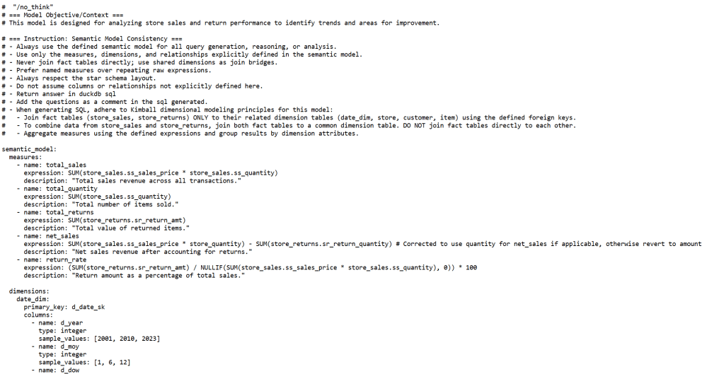
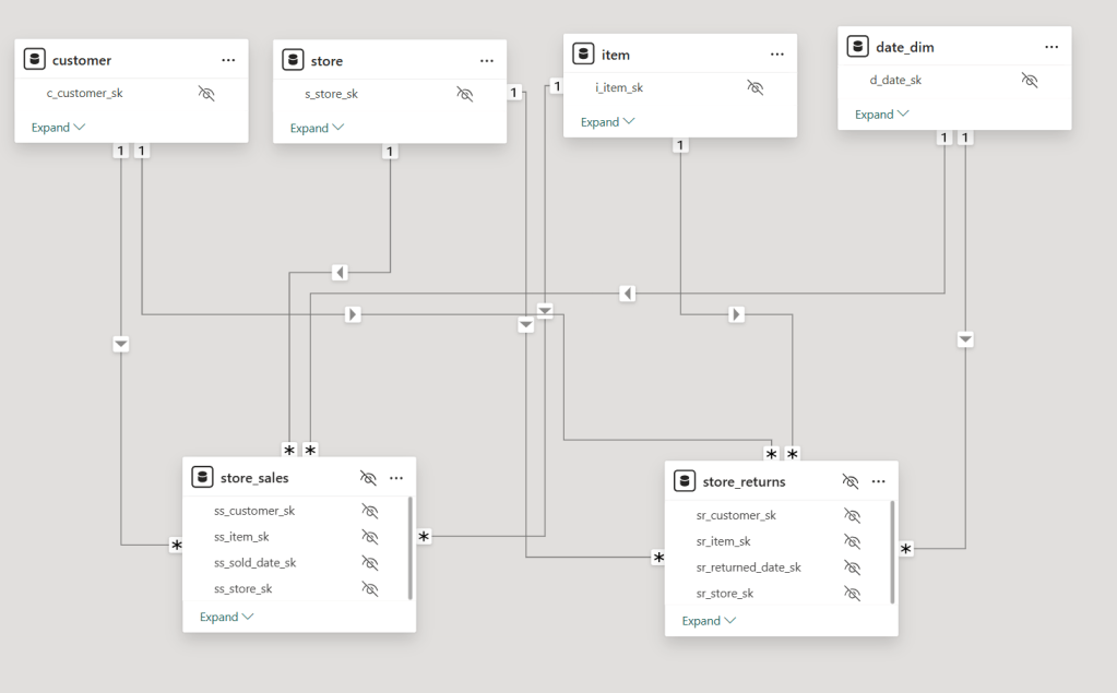
A semantic_model.txt file acts as the system prompt. This guides the model to produce more accurate and structured SQL outputs , the semantic model itself was generated by another LLM, it does include non trivial verified SQL queries ,sample values, relationships , measures etc, custom instructions

“no_think” is to turn off the thinking mode in Qwen3

1. Setup and Environment

  • The notebook expects an Ollama instance running locally, with the desired models (like qwen3:8b, qwen3:4b) already pulled using ollama run <model_name>.

2. How It Works

Two main functions handle the process:

  • get_ollama_response:
    This function takes your natural language question, combines it with the semantic prompt, sends it to the Local Ollama server, and returns the generated SQL.
  • execute_sql_with_retry:
    It tries to run the SQL in DuckDB. If the query fails (due to syntax or binding errors), it asks the model to fix it and retries—until it either works or hits a retry limit.

In short, you type a question, the model responds with SQL, and if it fails, the notebook tries to self-correct and rerun.

3. Data Preparation

The data was generated using a Python script with a scale factor (e.g., 0.1). If the corresponding DuckDB file didn’t exist, the script created one and populated it with the needed tables. Again, the idea was to keep things lightweight and portable.

Figure: Example semantic model

4. Testing Questions

Here are some of the questions I tested, some are simple questions others a bit harder and require more efforts from the LLM

  • “total sales”
  • “return rate”
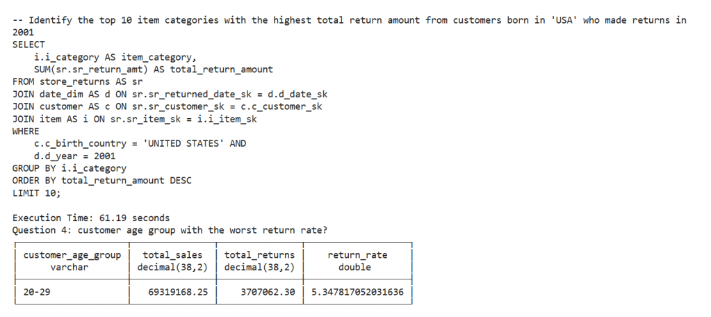
  • “Identify the top 10 item categories with the highest total return amount from customers born in ‘USA’ who made returns in 2001.”
  • “customer age group with the worst return rate?”
  • “return rate per year”
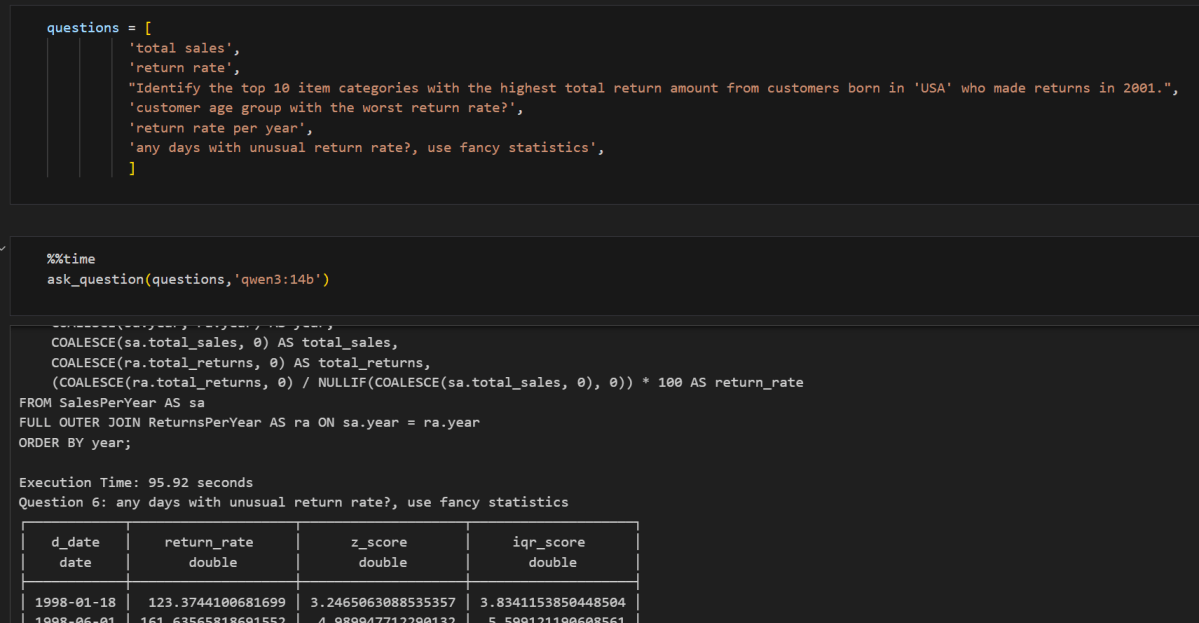
  • “any days with unusual return rate?, use fancy statistics”

Each question was sent to different models (qwen3:14b, qwen3:8b, qwen3:4b) to compare their performance. I also used %%time to measure how long each model took to respond, some questions were already in the semantic model, verified query answers, so in a sense it is a test too to see how the model stick with the instruction


5. What Came Out

For every model and question, I recorded:

  • The original question
  • Any error messages and retries
  • The final result (or failure)
  • The final SQL used
  • Time taken per question and total time per model

6. Observations

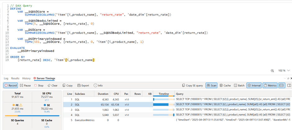
Question 6 : about detecting unusual return rates with “fancy statistics “stood out:

  • 8B model:
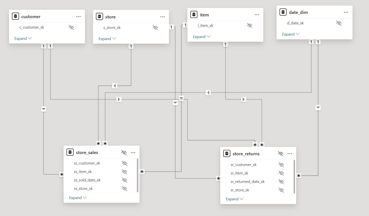
    Generated clean SQL using CTEs and followed a star-schema-friendly join strategy. No retries needed.
  • 14B model:
    Tried using Z-scores, but incorrectly joined two fact tables directly. This goes against explicit instruction in the semantic model.
  • 4B model:
    Couldn’t handle the query at all. It hit the retry limit without producing usable SQL.

By the way, the scariest part isn’t when the SQL query fails to run, it’s when it runs, appears correct, but silently returns incorrect results

Another behavior which I like very much, I asked a question about customers born in the ‘USA’, the model was clever enough to leverage the sample values and use ‘UNITED STATES’ instead in the filter.

Execution Times

  • 14B: 11 minutes 35 seconds
  • 8B: 7 minutes 31 seconds
  • 4B: 4 minutes 34 seconds

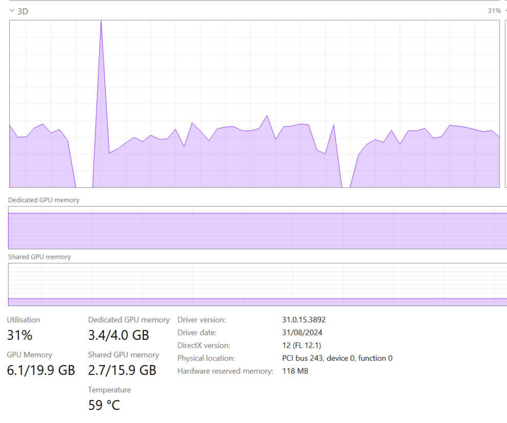
Tested on a laptop with 8 cores, 32 GB RAM, and 4 GB VRAM (Nvidia RTX A2000), the data is very small all the time is spent on getting the SQL , so although the accuracy is not too bad, we are far away from interactive use case using just laptop hardware.

7- Testing with simpler questions Only

I redone the test with 4B but using only simpler questions :

questions = [
          'total sales',
          'return rate',
          "Identify the top 10 item categories with the highest total return amount from customers born in 'USA' who made returns in 2001.",
          'return rate per year',
          'most sold items',
          ]
ask_question(questions,'qwen3:4b')

the 5 questions took less than a minutes, that promising !!!

Closing Thought

instead of a general purpose SLM, maybe a coding and sql fine tuned model with 4B size will be an interesting proposition, we live in an interesting time

Experimenting with Text-to-SQL: Lessons from Optimizing Product Return Analysis

🌟 Introduction

While testing the DuckDB ODBC driver, which is getting better and better (not production ready but less broken compared to two years ago), I noticed something unexpected. Running queries through Power BI in DirectQuery mode was actually faster than executing them directly in the DuckDB native UI.

Naturally, that does not make sense !!!

What followed was an investigation that turned into a fun and insightful deep dive into text-to-SQL generation, Power BI’s query behavior, and the enduring relevance of manual SQL tuning

🧩 The Goal: Find the Worst Product by Return Rate

The task was straightforward:

Calculate total sales, total returns, and return rate by product. Rank the products and find the top 5 with the highest return rates.

To make it interesting, I decided to try:

  1. Letting an LLM generate the SQL by loading the semantic model.
  2. Using PowerBI in Direct Query Mode.
  3. Finally, manually tuning the query.

📝 Step 1: LLM-generated SQL — Clean and Understandable

chatgpt generated a good starting point:

WITH sales_by_product AS   (
SELECT
i.i_product_name AS product_name,
SUM(ss.ss_sales_price * ss.ss_quantity) AS total_sales
FROM store_sales ss
JOIN item i ON ss.ss_item_sk = i.i_item_sk
WHERE i.i_product_name IS NOT NULL
GROUP BY i.i_product_name
),

returns_by_product AS (
SELECT
i.i_product_name AS product_name,
SUM(sr.sr_return_amt) AS total_returns
FROM store_returns sr
JOIN item i ON sr.sr_item_sk = i.i_item_sk
WHERE i.i_product_name IS NOT NULL
GROUP BY i.i_product_name
),

combined AS (
SELECT
COALESCE(s.product_name, r.product_name) AS product_name,
COALESCE(s.total_sales, 0) AS total_sales,
COALESCE(r.total_returns, 0) AS total_returns
FROM sales_by_product s
FULL OUTER JOIN returns_by_product r
ON s.product_name = r.product_name
)

SELECT
product_name,
ROUND((total_returns / NULLIF(total_sales, 0)) * 100, 2) AS return_rate
FROM combined
WHERE total_sales > 0 -- Avoid divide by zero
ORDER BY return_rate DESC
limit 5 ;

Pros:

  • Clean and easy to read.
  • Logically sound.
  • Good for quick prototyping.

🔍 Observation: However, it used product_name (a text field) as the join key in the combined table, initially I was testing using TPC-DS10, the performance was good, but when I changed it to DS100, performance degraded very quickly!!! I should know better but did not notice that product_name has a lot of distinct values.

the sales table is nearly 300 M rows using my laptop, so it is not too bad

and it is nearly 26 GB of highly compressed data ( just to keep it in perspective)

📊 Step 2: Power BI DirectQuery Surprises

Power BI automatically generate SQL Queries based on the Data Model, Basically you defined measures using DAX, you add a visual which generate a DAX query that got translated to SQL, based on some complex logic, it may or may not push just 1 query to the source system, anyway in this case, it did generated multiple SQL queries and stitched the result together.

🔍 Insight: Power BI worked exactly as designed:

  • It split measures into independent queries.
  • It grouped by product_name, because that was the visible field in my model.
  • And surprisingly, it was faster than running the same query directly in DuckDB CLI!

Here’s my screenshot showing Power BI results and DAX Studio:


🧩 Step 3: DuckDB CLI — Slow with Text Joins

Running the same query directly in DuckDB CLI was noticeably slower, 290 seconds !!!


⚙️ Step 4: Manual SQL Tuning — Surrogate Keys Win

To fix this, I rewrote the SQL manually:

  • Switched to item_sk, a surrogate integer key.
  • Delayed lookup of human-readable fields.

Here’s the optimized query:

WITH sales_by_product AS (
SELECT
ss.ss_item_sk AS item_sk,
SUM(ss.ss_sales_price * ss.ss_quantity) AS total_sales
FROM store_sales ss
GROUP BY ss.ss_item_sk
),

returns_by_product AS (
SELECT
sr.sr_item_sk AS item_sk,
SUM(sr.sr_return_amt) AS total_returns
FROM store_returns sr
GROUP BY sr.sr_item_sk
),

combined AS (
SELECT
COALESCE(s.item_sk, r.item_sk) AS item_sk,
COALESCE(s.total_sales, 0) AS total_sales,
COALESCE(r.total_returns, 0) AS total_returns
FROM sales_by_product s
FULL OUTER JOIN returns_by_product r ON s.item_sk = r.item_sk
)

SELECT
i.i_product_name AS product_name,
ROUND((combined.total_returns / NULLIF(combined.total_sales, 0)) * 100, 2) AS return_rate
FROM combined
LEFT JOIN item i ON combined.item_sk = i.i_item_sk
WHERE i.i_product_name IS NOT NULL
ORDER BY return_rate DESC
LIMIT 5;

🚀 Result: Huge performance gain! from 290 seconds to 41 seconds

Check out the improved runtime in DuckDB CLI:


🌍 In real-world models, surrogate keys aren’t typically used

unfortunately in real life, people still use text as a join key, luckily PowerBI seems to do better there !!!


🚀 Final Thoughts

LLMs are funny, when I asked chatgpt why it did not suggest a better SQL Query, I got this answer 🙂

I guess the takeaway is this:


If you’re writing SQL queries, always prefer integer types for your keys!

And maybe, just maybe, DuckDB (and databases in general) could get even better at optimizing joins on text columns. 😉

But perhaps the most interesting question is:
What if, one day, LLMs not only generate correct SQL queries but also fully performance-optimized ones?

Now that would be exciting.

you can download the data here, it is using very small factor : https://github.com/djouallah/Fabric_Notebooks_Demo/tree/main/SemanticModel

Edit : run explain analyze show that it is group by is taking most of the time and not the joins

the optimized query assumed already that i.i_item_sk is unique, it is not very obvious for duckdb to rewrite the query without knowing the type of joins !!! I guess LLMs still have a lot to learn

LLMs Are Getting Better at SQL

For no particular reason, I recently opened a Power BI report with two fact tables, exported the model definition to TMDL, saved it as a file, and loaded it into several state-of-the-art LLMs, including ChatGPT, Grok, Anthropic, and Qwen QWQ. I wasn’t particularly interested in comparing specific models—I just wanted to get a general sense of how they performed. To keep things simple, I used only the free tiers.

To my surprise, these models are getting really smart. They all recognized that the file represented a Power BI semantic model. They understood the concept of tables, columns, relationships, and measures, which was quite impressive.

You can download the Model here , i added a semantic Model as a text file in case you don’t have PowerBI

The Power of Semantic Models

Power BI, and before that PowerPivot, has supported multiple fact tables from day one. I remember the first time I used PowerPivot— a colleague showed me how to handle multiple fact tables: just don’t join fact to fact. Instead, use a common dimension, and everything will work fine. Back then, I had no idea about Kimball, multi-stage SQL queries, chasm trap etc. As a business user, I only cared that I got the correct results. It took me years to appreciate the ingenuity and engineering that went into making this work seamlessly. To me, this is an example of great product design: solve a very hard problem, and people will use it.

But this blog isn’t about Power BI and DAX—that’s a solved problem. Instead, I wanted to explore whether LLMs, by reading only metadata, could generate correct SQL queries for relatively complex questions.

Note: for people not familiar with TMDL, it is a human readable format of PowerBI semantic Model ( if human can read it, then LLMs will understand it too)

Testing LLMs with SQL Generation

I started with simple queries involving only one fact table, and the results were straightforward. The models correctly referenced measure definitions, avoiding column name hallucinations. Good news so far.

Things got more interesting when I asked for a query using a more complex measure, such as Net Sales:

Net Sales = [Total Sales] - [Total Returns]

This measure involves two tables: store_sales and store_returns.

Expected SQL Approach: Drilling Across

My expectation was that the models would use the Drilling Across technique. For example, when asked for net sales and cumulative sales by year and brand, a well-structured query would look like this:

  1. Compute total sales by year and brand.
  2. Compute total returns by year and brand.
  3. Join these results on year and brand.
  4. Calculate net sales as [Total Sales] - [Total Returns].
  5. Calculate cumulative Sales

Most LLMs generated a similar approach. Some required a hint (“don’t ever join fact to fact”), but the biggest issue was the final join. Many models defaulted to a LEFT JOIN, which is problematic—some returns for a brand might not occur in the same period as the sales, leading to incomplete results.

That said, some models got it right on the first attempt, which was very impressive. something like this:

WITH sales AS (
    SELECT
        d.d_year,
        i.i_brand,
        SUM(s.ss_sales_price * s.ss_quantity) AS total_sales
    FROM store_sales s
    JOIN item i ON s.ss_item_sk = i.i_item_sk
    JOIN date_dim d ON s.ss_sold_date_sk = d.d_date_sk
    GROUP BY d.d_year, i.i_brand
),
returns AS (
    SELECT
        d.d_year,
        i.i_brand,
        SUM(r.sr_return_amt) AS total_returns
    FROM store_returns r
    JOIN item i ON r.sr_item_sk = i.i_item_sk
    JOIN date_dim d ON r.sr_returned_date_sk = d.d_date_sk
    GROUP BY d.d_year, i.i_brand
)
SELECT
    COALESCE(s.d_year, r.d_year) AS year,
    COALESCE(s.i_brand, r.i_brand) AS brand,
    COALESCE(s.total_sales, 0) AS total_sales,
    COALESCE(r.total_returns, 0) AS total_returns,
    (COALESCE(s.total_sales, 0) - COALESCE(r.total_returns, 0)) AS net_sales,
    SUM(COALESCE(s.total_sales, 0) - COALESCE(r.total_returns, 0))
        OVER (PARTITION BY COALESCE(s.i_brand, r.i_brand) ORDER BY COALESCE(s.d_year, r.d_year)
        ROWS BETWEEN UNBOUNDED PRECEDING AND CURRENT ROW) AS cumulative_net_sales
FROM sales s
FULL OUTER JOIN returns r
ON s.d_year = r.d_year AND s.i_brand = r.i_brand
ORDER BY COALESCE(s.i_brand, r.i_brand), COALESCE(s.d_year, r.d_year);

An Alternative Approach: UNION ALL

One LLM got creative and proposed a different solution using UNION ALL:

WITH combined AS (
    SELECT d.d_year, i.i_brand, 'sales' AS type, s.ss_sales_price * s.ss_quantity AS amount
    FROM store_sales s
    JOIN date_dim d ON s.ss_sold_date_sk = d.d_date_sk
    JOIN item i ON s.ss_item_sk = i.i_item_sk
    UNION ALL
    SELECT d.d_year, i.i_brand, 'returns' AS type, r.sr_return_amt AS amount
    FROM store_returns r
    JOIN date_dim d ON r.sr_returned_date_sk = d.d_date_sk
    JOIN item i ON r.sr_item_sk = i.i_item_sk
)
SELECT
    d_year AS year,
    i_brand AS brand,
    SUM(CASE WHEN type = 'sales' THEN amount ELSE 0 END) AS total_sales,
    SUM(CASE WHEN type = 'returns' THEN amount ELSE 0 END) AS total_returns,
    (SUM(CASE WHEN type = 'sales' THEN amount ELSE 0 END) - SUM(CASE WHEN type = 'returns' THEN amount ELSE 0 END)) AS net_sales,
    SUM(SUM(CASE WHEN type = 'sales' THEN amount ELSE 0 END) - SUM(CASE WHEN type = 'returns' THEN amount ELSE 0 END))
        OVER (PARTITION BY i_brand ORDER BY d_year ROWS BETWEEN UNBOUNDED PRECEDING AND CURRENT ROW) AS cumulative_net_sales
FROM combined
GROUP BY d_year, i_brand
ORDER BY i_brand, d_year;

Edit : people who know what they are doing , did not like the union all solution for performance reason

So, Is SQL a Solved Problem?

No, of course not. There’s still no guarantee of getting the same answer when asking the same question multiple times. Additionally, AI has no real understanding of the data. The moment you introduce filters, you can get all sorts of unexpected results,Although Providing sample values from columns into a semantic model helps a lot, still real-world models are far more complex and often contain ambiguities.

While LLMs generate correct SQL, they don’t always generate the most efficient queries, But you can argue, it is the Database problem to solve 🙂

Compute Considerations

I don’t know enough to make a strong statement about the current cost of running LLMs, but I ran a simple experiment: I tested QWQ-32 on my laptop (which has an NVIDIA RTX A2000 GPU with 4GB of dedicated memory). The good news? It worked. Running an open-source “thinking model” on a personal laptop is already impressive. The bad news? It was painfully slow—so much so that I’m not eager to repeat the test.

From a practical perspective, generating SQL queries this way seems extremely expensive. A decent BI tool can generate similar queries in milliseconds, using orders of magnitude less compute power, but as LLMs continue to improve in efficiency, maybe in a couple of years, the compute requirement to generate SQL Queries will become trivial ?

Final Thoughts

Having experimented with LLMs since 2023, I can say with confidence that they have improved significantly ( LLMs in 2023 were not very good to be honest). They are getting better and, more importantly, cheaper, opening the door for new applications.

The initial promise was that you could just throw data at an AI system, and it would figure out everything. I suspect that’s not true. In reality, to get useful results, you need more structure, and well-defined semantic models will play a crucial role in making asking your Data a reality.

Building Idempotent Data Pipelines with DuckDB SQL

Alright using the term “idempotent” was just a clickbait 🙂 it simply means avoiding the processing of the same file multiple times ( ok for a formal definition wikipedia has a nice article). in this case the script will process only new files added to the source system, assuming the filenames are unique.

Although this is easily accomplished using Python API , achieving the same result using DuckDB SQL was a bit tricky until the introduction of SQL variables in the developpement branch a couple of weeks ago, particularly Variables can now be referenced within read files operation.

in summary this is what the SQL script is doing.

  1. Creation of a Hive table in the file section of onelake, it is very important step, if you query an empty folder you will get an error, , as DuckDB does not support external table, we will just add a dummy parquet file with empty rows, it is filtered out in the next step.
  COPY (
  SELECT
    '' AS filename,
    NULL AS year ) TO "/lakehouse/default/Files/scada" (FORMAT PARQUET,
    PARTITION_BY (year),
    OVERWRITE_OR_IGNORE ) ;
  1. Listing of CSV files for ingestion from the source system.
  2. Removal of already ingested files
SET
  VARIABLE list_of_files = (
  SELECT
    list(file)
  FROM
    glob("/lakehouse/default/Files/Daily_Reports/*.CSV")
  WHERE
    parse_filename(file) NOT IN (
    SELECT
      filename
    FROM
      read_parquet("/lakehouse/default/Files/scada/*/*.parquet")))
  1. Generate list of new files and pass it to DuckDB for processing.

just a preview of the query plan for this step

  1. Saving as partitioned Hive parquet folders

Note : I am using Fabric notebook as an example, but obviously you can run it anywhere, actually I did it run in my laptop and as far as I can tell, Onelake throughput is competitive with my ssd disk 🙂

  COPY (
  SELECT
    '' AS filename,
    NULL AS year ) TO "/lakehouse/default/Files/scada" (FORMAT PARQUET,
    PARTITION_BY (year),
    OVERWRITE_OR_IGNORE ) ;
SET
  VARIABLE list_of_files = (
  SELECT
    list(file)
  FROM
    glob("/lakehouse/default/Files/Daily_Reports/*.CSV")
  WHERE
    parse_filename(file) NOT IN (
    SELECT
      filename
    FROM
      read_parquet("/lakehouse/default/Files/scada/*/*.parquet"))) ;
CREATE OR REPLACE VIEW
  raw AS (
  SELECT
    *
  FROM
    read_csv(getvariable('list_of_files'),
      Skip=1,
      header =0,
      all_varchar=1,
      COLUMNS={ 'I': 'VARCHAR',
      'UNIT': 'VARCHAR',
      'XX': 'VARCHAR',
      'VERSION': 'VARCHAR',
      'SETTLEMENTDATE': 'VARCHAR',
      'RUNNO': 'VARCHAR',
      'DUID': 'VARCHAR',
      'INTERVENTION': 'VARCHAR',
      'DISPATCHMODE': 'VARCHAR',
      'AGCSTATUS': 'VARCHAR',
      'INITIALMW': 'VARCHAR',
      'TOTALCLEARED': 'VARCHAR',
      'RAMPDOWNRATE': 'VARCHAR',
      'RAMPUPRATE': 'VARCHAR',
      'LOWER5MIN': 'VARCHAR',
      'LOWER60SEC': 'VARCHAR',
      'LOWER6SEC': 'VARCHAR',
      'RAISE5MIN': 'VARCHAR',
      'RAISE60SEC': 'VARCHAR',
      'RAISE6SEC': 'VARCHAR',
      'MARGINAL5MINVALUE': 'VARCHAR',
      'MARGINAL60SECVALUE': 'VARCHAR',
      'MARGINAL6SECVALUE': 'VARCHAR',
      'MARGINALVALUE': 'VARCHAR',
      'VIOLATION5MINDEGREE': 'VARCHAR',
      'VIOLATION60SECDEGREE': 'VARCHAR',
      'VIOLATION6SECDEGREE': 'VARCHAR',
      'VIOLATIONDEGREE': 'VARCHAR',
      'LOWERREG': 'VARCHAR',
      'RAISEREG': 'VARCHAR',
      'AVAILABILITY': 'VARCHAR',
      'RAISE6SECFLAGS': 'VARCHAR',
      'RAISE60SECFLAGS': 'VARCHAR',
      'RAISE5MINFLAGS': 'VARCHAR',
      'RAISEREGFLAGS': 'VARCHAR',
      'LOWER6SECFLAGS': 'VARCHAR',
      'LOWER60SECFLAGS': 'VARCHAR',
      'LOWER5MINFLAGS': 'VARCHAR',
      'LOWERREGFLAGS': 'VARCHAR',
      'RAISEREGAVAILABILITY': 'VARCHAR',
      'RAISEREGENABLEMENTMAX': 'VARCHAR',
      'RAISEREGENABLEMENTMIN': 'VARCHAR',
      'LOWERREGAVAILABILITY': 'VARCHAR',
      'LOWERREGENABLEMENTMAX': 'VARCHAR',
      'LOWERREGENABLEMENTMIN': 'VARCHAR',
      'RAISE6SECACTUALAVAILABILITY': 'VARCHAR',
      'RAISE60SECACTUALAVAILABILITY': 'VARCHAR',
      'RAISE5MINACTUALAVAILABILITY': 'VARCHAR',
      'RAISEREGACTUALAVAILABILITY': 'VARCHAR',
      'LOWER6SECACTUALAVAILABILITY': 'VARCHAR',
      'LOWER60SECACTUALAVAILABILITY': 'VARCHAR',
      'LOWER5MINACTUALAVAILABILITY': 'VARCHAR',
      'LOWERREGACTUALAVAILABILITY': 'VARCHAR' },
      filename =1,
      null_padding = TRUE,
      ignore_errors=1,
      auto_detect=FALSE)
  WHERE
    I='D'
    AND UNIT ='DUNIT'
    AND VERSION = '3' ) ; COPY (
  SELECT
    UNIT,
    DUID,
    parse_filename(filename) AS filename,
    CAST(COLUMNS(*EXCLUDE(DUID,
          UNIT,
          SETTLEMENTDATE,
          I,
          XX,
          filename)) AS double),
    CAST (SETTLEMENTDATE AS TIMESTAMPTZ) AS SETTLEMENTDATE,
    isoyear (CAST (SETTLEMENTDATE AS timestamp)) AS year
  FROM
    raw) TO "/lakehouse/default/Files/scada" (FORMAT PARQUET,
    PARTITION_BY (year),
    APPEND ) ;

While the Python API in a notebook is IMHO  the easiest approach for data transformation, it is nice to see that Pure SQL can support it. 

However, the real game-changer will be when DuckDB introduces support for Delta write. for now, you need another step to load those Parquet files to Delta either using Deltalake Python package or Spark Delta writer.