Fabric for Small Enterprises

While experimenting with different access modes in Power BI, I thought it is maybe worth sharing as a  short blog to show  why the Lakehouse architecture offers versatile options for Power BI developers. Even when they use Only Import Mode. 

And Instead of sharing a conceptual piece, perhaps focus on presenting some dollar figures 🙂

Scenario: A Small Consultancy

According to local regulations, a small enterprise is defined as having fewer than 15 employees. Let’s consider this setup:

  • Data Storage: The data resides in Microsoft OneLake, utilizing an F2 SKU.
  • Number of Users: 15 employees.
  • Data Size: Approximately 94 million rows.
  • Pricing Model: For simplicity, assume the F2 SKU uses a reserved pricing model.

Monthly Costs:

  • Power BI Licensing: 15 users × 15 AUD = 225 AUD.
  • F2 SKU Reserved Pricing: 293 AUD.
  • Total Cost: 518 AUD per month.

ETL Workload

Currently, the ETL workload consumes approximately 50% of the available capacity.

 For comparison, I ran the same workload on another Lakehouse vendor. To minimize costs, the schedule was adjusted to operate only from 8 AM to 6 PM. Despite this adjustment, the cost amounted to:

  • Daily Cost: 40 AUD.
  • Monthly Cost: 1,200 AUD.

In contrast, the F2 SKU’s reserved price of 293 AUD per month is significantly more economical. Even the pay-as-you-go model, which costs 500 AUD per month, remains competitive.

Key Insight:

While serverless billing is attractive, what matter is how much you end up paying per month.

For smaller workloads (less than 100 GB of data), data transformation becomes commoditized, and charging a premium for it is increasingly challenging.

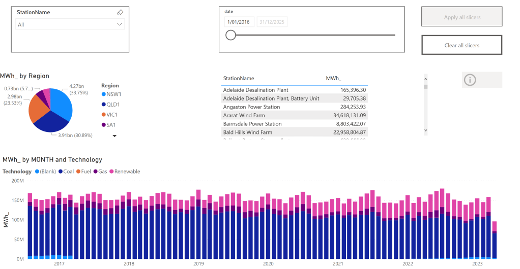
Analytics in Power BI

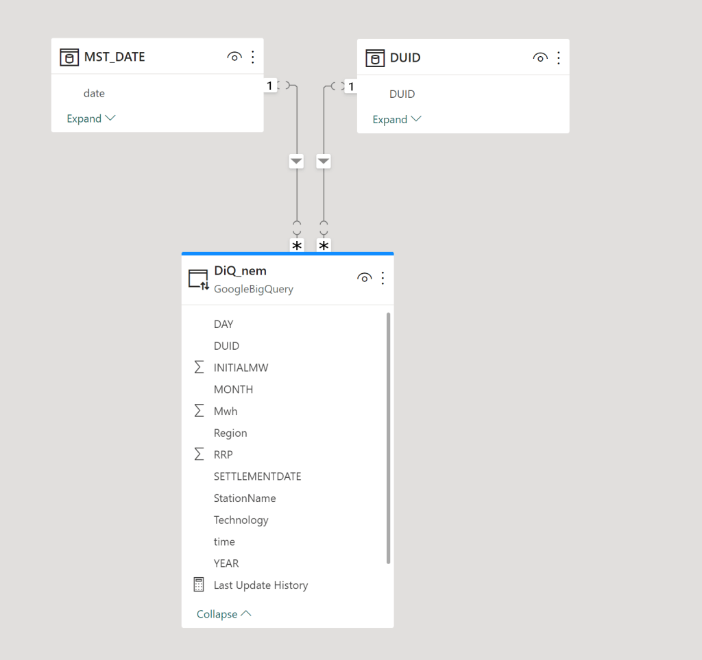
I prefer to separate Power BI reports from the workspace used for data transformation. End users care primarily about clean, well-structured tables—not the underlying complexities.

With OneLake, there are multiple ways to access the stored data:

  1. Import Mode: Directly import data from OneLake.
  2. DirectQuery: Use the Fabric SQL Endpoint for querying.
  3. Direct Lake Model: Access data with minimal latency.
  4. Composite Models: All the above ( this is me trying to be funny) 

All the Semantic Models and reports are hosted in the Pro license workspace, Notice that an import model works even when the capacity is suspended ( if you are using pay as you go pricing)

The Trade-Off Triangle

In analytical databases, including Power BI, there is always a trade-off between cost, freshness, and query latency. Here’s a breakdown:

  • Import Mode: Ideal if eight refreshes per day suffice and the model size is small. Reports won’t consume Fabric capacity (Onelake Transactions cost are insignificant for small data import)
  • Direct Lake Model: Provides excellent freshness and latency but will probably impacts F2 capacity, in other words, it will cost more.
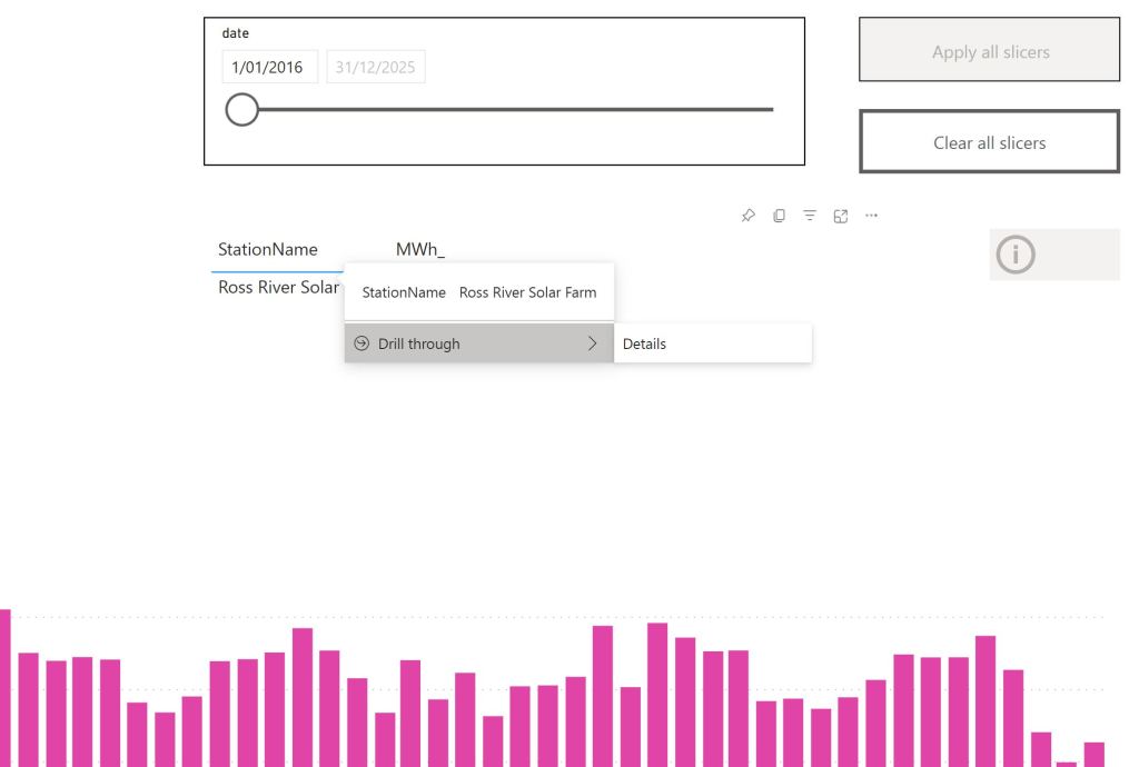
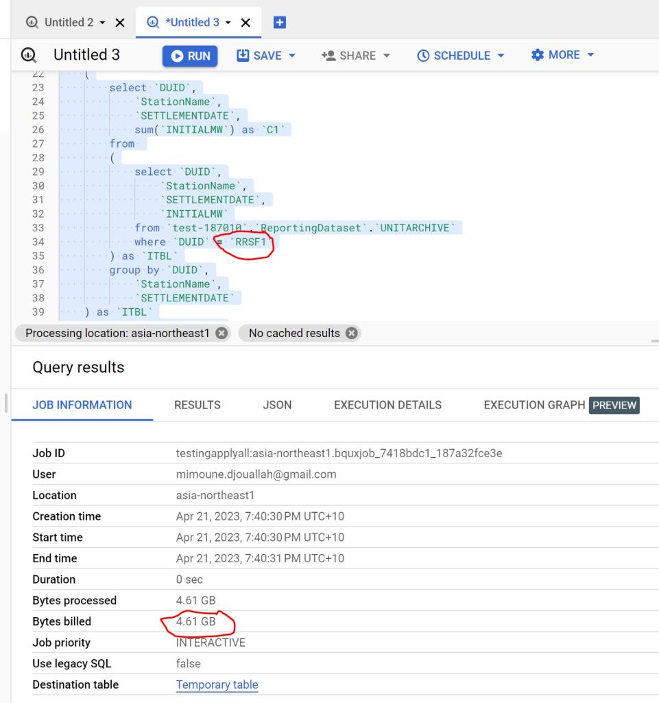
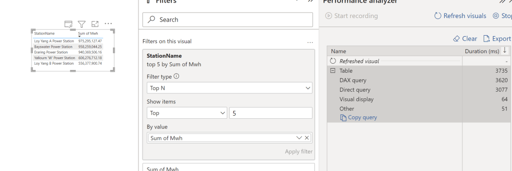
  • DirectQuery: Balances freshness and latency (seconds rather than milliseconds) while consuming less capacity. This approach is particularly efficient as Fabric treats those Queries as background operations, with low consumption rates in many cases. Looking forward to the release of Fabric DWH result cache. 

Key Takeaways

  1. Cost-Effectiveness: Reserved pricing for smaller Fabric F SKUs combined with Power BI Pro license offers a compelling value proposition for small enterprises.
  2. Versatility: OneLake provides flexible options for ETL workflows, even when using import mode exclusively.

The Lakehouse architecture and Power BI’s diverse access modes make it possible to efficiently handle analytics, even for smaller enterprises with limited budgets.

Optimize BigQuery cost by creating independent sort order for the same table

TL;DR

Using materialized view to create a different sort order of the base table can reduce cost substantially, in this example up to 200 X for some queries.

The Problem : You can’t have multiple sort order.

One of most effective technique in columnar database to improve speed is to sort the table which will help the engine scan less data, but what if you have some queries that works better with different sorting, obviously you can’t have independent column sorted in the same table , turn out BigQuery has a very nice functionality, Materialized views which are used mainly to aggregate Data, see example here, can also works fine without aggregation and you can even change the sort order of the base table.

Example using PowerBI

In this report, which show analyze Electricity production for the Australian Market, the base table is sorted by day, that make perfect sense as most uses will want to see only a specific time period then aggregate by some attribute like region, technology etc

The Model is very simple , a fact table in Direct Query mode, and two dimensions in Import mode, a very simple star schema

The main report is a couple of charts using some aggregation, nothing particularly interesting, the queries use the Materialized view as we are aggregating per day, the base table is by minutes.

Drill Down to details

The trouble start here, let’s say a user want to see all the data for one particular Station name to the lowest level of details.

The Engine will have to scan the full table, as the table was sorted by date not by Station name

as you can see 4.61 GB is a lot of data scanned just to see one station name.

Non Aggregation Materialized View

let’s create a new MV with a different sort order, notice there is no group by, it is the same number of rows as the base table and you can’t have different partitions, only sort can be changed.

create  materialized view `XXX_MV_Sort`
cluster by   DUID,DAY as 

SELECT
  *
FROM
  BASE_Table

The Same Query is substantially cheaper 🙂 from 4.6 GB to 19 MB, that’s 230 times cheaper.

you can see the two Query Plan, one scanning 101 Millions rows vs 404000 rows

Take away

Because BigQuery already knows about all the queries, it may be useful to have some kind of service that give suggestions, like changing sort or adding a Materialized view, in the meantime, I think Modeling still matter and can save you a lot of money.

PowerBI Query plan when using Top N filter

The October release of PowerBI Desktop introduced a very interesting feature, Top N filtered is pushed down for Direct Query Sources, I thought I may give it a try and blog about it, for some reason it did not work, which is great for the purpose of this blog as if you came from a SQL Background you will be surprised how PowerBI DAX Engine Works.

let’s try with one table in BigQuery as an example, and ask this Question, what’s the top 5 Substation by Electricity produced, in PowerBI, it is a trivial exercise, just use the Top N filter

First Observation, 3.7 Second seems rather Slow, BigQuery or any Columnar Database should return the results way faster, specially that we are grouping by low cardinality columns ( around 250 distinct values)

Let’s try SQL Query in BigQuery Console

And let’s check the duration, 351 ms, the table has 91 Million records, that’s not bad at all, but we need to account for the data transfer latency to my laptop, still that does not explain the difference in duration !!!

DAX Engine Query Plan

let’s have a look at the Query Plan generated by DAX Engine using the excellent free tool, DAX Studio

That’s very strange, 2 SQL Query and 1 Second spent by the Formula Engine, and the two SQL Queries are not even in parallel

Looking at the SQL Queries, I think this is the logic of the Query Plan

  • Send a SQL Query to get the list of all the substation and the sum of of MWH.
  • Order the result using the Formula Engine and select 5 substation.
  • Send another SQL Query with a filter of those 5 substation

Probably you are wondering why this convoluted Query Plan, Surely DAX Engine can just send 1 SQL Query to get the results, why the two trips to the source system, which make the whole experience slow.

Vertipaq Don’t support Sort Operator

Vertipaq which is the internal storage engine of PowerBI does not support the sort operator, hence the previous Query do make sense if your Storage engine don’t support sort.

But My Source do support Sorting ?

That’s the new feature, DAX Engine will generate a different plan when the source system do support sorting.

Great, again , Why Vertipaq don’t support sort Operator ?

No idea, probably only a couple of engineers from Microsoft Know the answer.

Edit : 23 October 2022

Jeffrey Wang ( One of the Original Authors of DAX Engine) was very kind and provided this explanation why the optimization did not kick in for BigQuery

Query Performance in Vertipaq vs DuckDB

Edit : this blog generated some strong feedback, This is not a benchmark of Vertipaq, but rather me arguing that it is indeed possible to have a good enough OLAP SQL Engine that read from disk instead of RAM ?

Vertipaq is the columnar Database used In PowerBI, Excel and Analysis service, it is an extremely fast DB and I have being using it since 2015 without really understanding how it works, it is just there giving back results in sub second, the only time I got performance issue was when I wrote terribly bad DAX.

Just for fun and hopefully we may even learn something useful, I run a couple of simple SQL Queries in DuckDB and replicate them in PowerBI desktop and see how the two system behave,Unfortunately Vertipaq don’t expose a fully functional SQL Endpoint, so you can’t simply run a typical SQL benchmark.

Setup

All test were done using my laptop ( a Dell with 16 GB of RAM), the data is TPCH-SF10, 60 million of rows for the base table, I had to add a PK for PowerBI as it does not support join on multiple fields, you can download the raw Data here

DuckDB queries were run using Visual studio notebook, I would had prefered Malloy but it does not support native DuckDB storage format yet , you can download the python files here and how to create the DB and Tables

For PowerBI, I use DAX Studio with cache turned off.

Loading Data

DuckDB support multiple mode, you can just run Queries directly on parquet files, you can load the data to memory using temp tables or you can import the data using DuckDB storage format, for performance reason I import the data, DuckDB don’t support compression very well yet, and consider the storage format as a work in progress, Index currently are not compressed and take a lot of space, without index, the size is around 3.6 GB

Parquet : 2.9 GB

DuckDB storage file format : 17 GB

Vertipaq : 3.9 GB

Notice here, DuckDB is reading from disk to run Queries, if does filter pushdown and scan only column used in Queries, Vertipaq has to load the whole database into memory before you can run any Queries, as far as I can tell this is the most important difference between the two systems and has a massive implication, both positive and negative.

Data Model

I am using the same Data Model as the previous blog, it is a nice bad Model for testing 🙂

1- Simple Count Distinct

DuckDB : 4.4 S

Vertipaq : 0 S

For vertipaq it is a metadata Query, the distinct count for a whole column is created when you import the data, DuckDB don’t save that particular statistic.

2- Count Distinct group by low Cardinality

low cardinality simply means column with small number of unique values.

DuckDB : 10.8 S

Vertipaq : 7.1 S

3- Count Distinct group by high Cardinality

now count the distinct values but grouping by a column L_comments which contains 33 Million unique values

DuckDB : 49 S

Vertipaq : 29 S

4 – Sum group by low Cardinality

This one is using the Famous Query 1 of TPCH Benchmark

DuckDB : 0.7 S

Vertipaq : 0.3 S

5 – Sum group by high Cardinality

DuckDB : 2.7 S

Vertipaq : 17 S

6 – Aggregate using complex relationship but group by Low cardinality

The performance of Vertipaq keep surprising me, it is using some kind of index on joins, I don’t know really how it works, but the performance is impressive

DuckDB : 4.9 S

Vertipaq : 0.9 S

7 – Aggregate using complex relationship but group by High cardinality

DuckDB : 8.4 S

Vertipaq : 5.1 S

I was surprised by this results, it seems when you group by high cardinality column it will impact Vetipaq performance.

8 – Aggregate and filter on Text

DuckDB : 3.1 S

Vertipaq : 58 S

The performance seems odd for vertipaq, maybe I am doing something wrong, but it should be straightforward

Edit : Alex was kind enough and provided this excellent explanation.

9- Count Distinct group by high Cardinality base Table 120 Million records

Basically that’s the point of the blog, yes Vertipaq works well because it does fit into my Laptop RAM, let’s try a complex Query using 120 Million ? I start getting memory errors

Actually the whole experience became sluggish, just saving any edits take ages.

Let’s try DuckDB, I will just Query from parquet, I don’t want to ingest 120 million records for one Query

Take Away

here is the summary results

Vertipaq is extremely fast but the performance degrade when dealing with High cardinality columns, filtering using string seems slow though, the Index on join or whatever the engine is doing is genius, the result for the Query 4 and 6 are magic as far as I am concerned.

DuckDB is impressive especially with the fact it is reading from Disk, yes, it is slower than Vertipaq for a small Data size which is expected as generally speaking scanning from RAM will be faster than Disk, but it does scale better.

If your data don’t fit into the RAM, DuckDB seems like an interesting proposition.