it is a quick post on how to query Onelake Iceberg REST Catalog using pure SQL with DuckDB, and yes you need a service principal that has access to the lakehouse
it works reasonably well assuming your region is not far from your laptop, or even better , if you run it inside Fabric then there is no network shenanigans, I recorded a video showing my experience
Why read operations do not always need full consistency checks
I hope DuckDB eventually adds an option that allows turning off table state checks for purely read scenarios. The current behaviour is correct because you always need the latest state when writing in order to guarantee consistency. However, for read queries it feels unnecessary and hurts the overall user experience. PowerBI solved this problem very well with its concept of framing, and something similar in DuckDB would make a big difference, notice duckdb delta reader already support pin version.
While preparing for a presentation about the FabCon announcement, one item was about OneLake Diagnostics. all ll I knew was that it had something to do with security and logs. As a Power BI user, that’s not exactly the kind of topic that gets me excited, but I needed to know at least the basic, so I can answer questions if someone ask 🙂
Luckily, we have a tradition at work , whenever something security-related comes up, we just ping Amnjeet🙂
He showed me how it works , and I have to say, I loved it. It’s refreshingly simple.
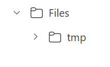
You just select a folder in your Lakehouse and turn it on.
That’s it , the system automatically starts generating JSON files, neatly organized using Hive-style partitions, By default, user identity and IP tracking are turned off unless an admin explicitly enables them. You can find more details about the schema and setup here.
What the Logs Look Like
Currently, the logs are aggregated at the hourly level, but the folder structure also includes a partition for minutes (even though they’re all grouped at 00 right now).
Parsing the JSON Logs
Once the logs were available, I wanted to do some quick analysis , not necessarily about security, just exploring what’s inside.
There are probably half a dozen ways to do this in Fabric ; Shortcut Transform, RTI, Dataflow Gen2, DWH, Spark, and probably some AI tools too, Honestly, that’s a good problem to have.
But since I like Python notebooks and the data is relatively small, I went with DuckDB (as usual), but Instead of using plain DuckDB and delta_rs to store the results, I used my little helper library, duckrun, to make things simpler ( Self Promotion alert).
Then I asked Copilot to generate a bit of code for registering existing functions to look up the workspace name and lakehouse name from their GUIDs in DuckDB, using SQL to call python is cool 🙂
The data is stored incrementally, using the file path as a key , so you end up with something like this:
Then I added only the new logs with this SQL script:
try:
    con.sql(f"""
        CREATE VIEW IF NOT EXISTS logs(file) AS SELECT 'dummy';
        SET VARIABLE list_of_files =
        (
            WITH new_files AS (
                SELECT file
                FROM glob('{onelake_logs_path}')
                WHERE file NOT IN (SELECT DISTINCT file FROM logs)
                ORDER BY file
            )
            SELECT list(file) FROM new_files
        );
        SELECT * EXCLUDE(data), data.*, filename AS file
        FROM read_json_auto(
            GETVARIABLE('list_of_files'),
            hive_partitioning = true,
            union_by_name = 1,
            FILENAME = 1
        )
    """).write.mode("append").option("mergeSchema", "true").saveAsTable('logs')
except Exception as e:
    print(f"An error occurred: {e}")
1- Using glob() to collect file names means you don’t open any files unnecessarily , a small but nice performance win.
2- DuckDB expand the struct using this expression data.*
3- union_by_name = 1 in case the json has different schemas
4- option(“mergeSchema”, “true”) for schema evolution in Delta table
Exploring the Data
Once the logs are in a Delta table, you can query them like any denormalize table.
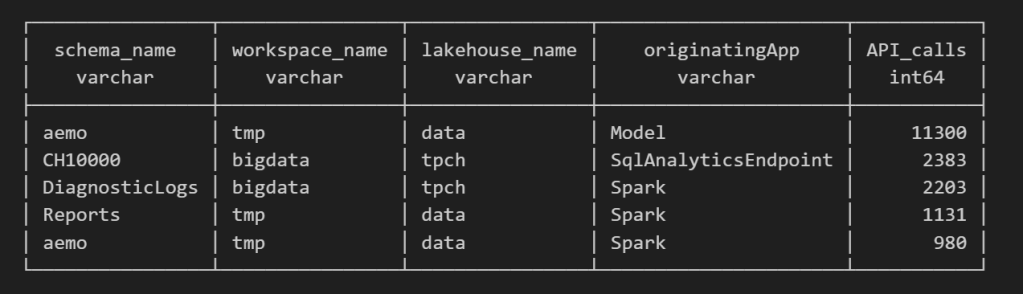
For example, here’s a simple query showing API calls per engine:
Note : using AI to get working regex is maybe the best thing ever 🙂
SELECT
    regexp_extract(resource, '([^&/]+)/([^&/]+)/(Tables|Files)(?:/([^&/]+))?(?:/([^&/]+))?', 4) AS schema_name,
    get_workspace_name(workspaceid) AS workspace_name,
    get_lakehouse_name(workspaceid, itemId) AS lakehouse_name,
    originatingApp,
    COUNT(*) AS API_calls
FROM logs
GROUP BY ALL
ORDER BY API_calls DESC
LIMIT 5;
Fun fact: OneLake tags Python notebook as Spark. Also, I didn’t realize Lineage calls OneLake too!
as I have already register Python functions as UDFs, which is how I pulled in the workspace and lakehouse names in the query above.
Takeaway
This was just a bit of tinkering, but I’m really impressed with how easy OneLake Diagnostics is to set up and use.
I still remember the horrors of trying to connect Dataflow Gen1 to Azure Storage ,that was genuinely painful (and I never even got access from IT anyway).
It’s great to see how Microsoft Fabric is simplifying these scenarios. Not everything can always be easy, but making the first steps easy really gives the feature a very good impression.
This started as just a fun experiment. I was curious to see what happens when you push DuckDB really hard — like, absurdly hard. So I went straight for the biggest Python single-node compute we have in Microsoft Fabric: 64 cores and 512 GB of RAM. Because why not?
Setting Things Up
I generated data using tpchgenand registered it with delta_rs. Both are Rust-based tools, but I used their Python APIs (as it should be, of course). I created datasets at three different scales: 1 TB, 3 TB, and 10 TB.
From previous tests, I know that Ducklake works better, but I used Delta so it is readable by other Fabric Engines ( as of this writing , Ducklake does not supporting exporting Iceberg metadata, which is unfortunate)
The goal wasn’t really about performance . I wanted to see if it would work at all. DuckDB has a reputation for being great with smallish data, but wanted to see when the data is substantially bigger than the available Memory.
And yes, it turns out DuckDB can handle quite a bit more than most people assume.
The Big Lesson: Local Disk Matters
Here’s where things got interesting.
If you ever try this yourself, don’t use a Lakehouse folder for data spilling. It’s painfully slow(as the data is first written to disk then uploaded to remote storage)
Instead, point DuckDB to the local disk that Fabric uses for AzureFuse caching. That disk is about 2 TB. or any writable folder
You can tell DuckDB to use it like this:
SET temp_directory = '/mnt/notebookfusetmp';
Once I did that, I could actually see the data spilling happening in real time which felt oddly satisfying, it works but slow , it is better to just have more RAM 🙂
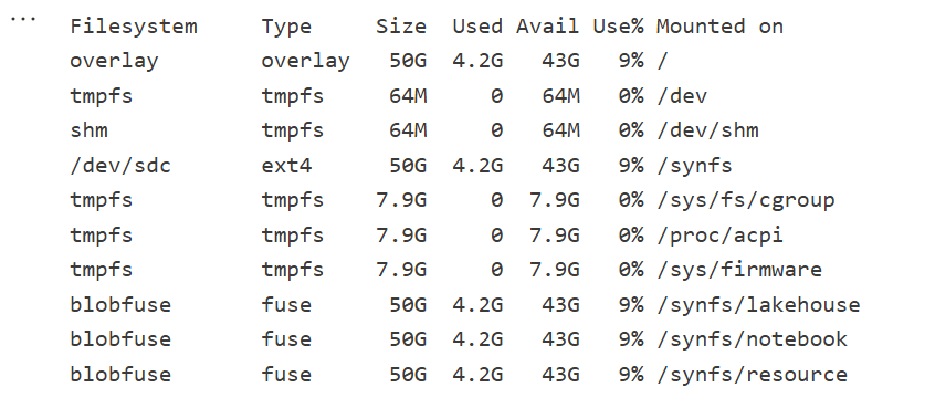
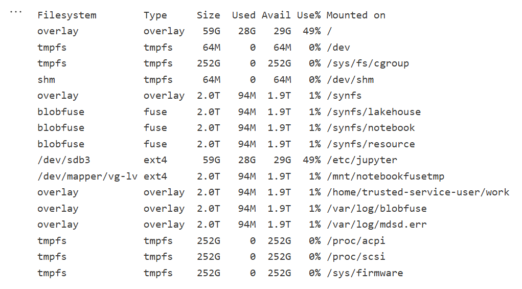
Python notebook is fundamentally just a Linux VM, and you can see the storage layout using this command
!df -hT
Here is the layout for 2 cores
Which is different when running it for 64 cores ( container vs VM, something like that), I notice the local disk increased with more cores, which make sense
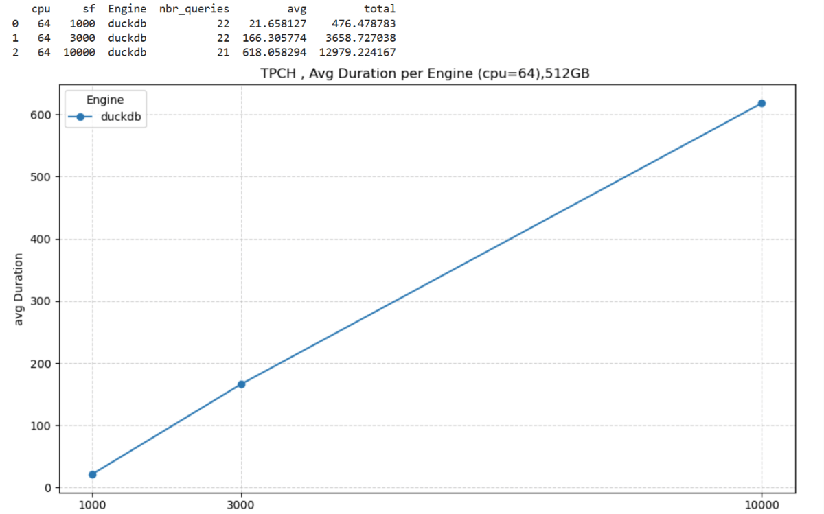
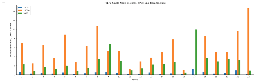
The Results
Most queries went through without too much trouble. except Query 17 at 10 TB scale? That one It ran for more than an hour before my authentication token expired. So technically, it didn’t fail 🙂
DuckDB does not have a way to refresh Azure token mid query. as far as I know
Edit : according to Claude, I need at least 1-2 TB of RAM (10-20% of database size) to avoid disk thrashing
Observations: DuckDB’s Buffer Pool
Something I hadn’t noticed before is how the buffer pool behaves when you work with data way bigger than your RAM. It tends to evict data that was just read from remote storage — which feels wasteful. I can’t help but think it might be better to spill that to disk instead.
I’m now testing an alternative cache manager called duck-read-cache-fs to see if it handles that better. We’ll see, i still think it is too low level to be handled by an extension, I know MotherDuck rewrote their own buffer manager, but not sure if it is for the same reason.
Why not test other Engines
I did, actually , and the best result I got was with Lakesail at around 100 GB. Beyond that, no single-node open-source engine can really handle this scale. Polars, for instance, doesn’t support spilling to disk at all and implements fewer than 10 of the 22 standard SQL queries.
Wrapping Up
So, what did I learn? DuckDB is tougher than it looks. With proper disk spilling and some patience, it can handle multi-terabyte datasets just fine, and sometimes the right solution is just to add more RAM
personally , I never had a need for TB of data ( my sweet spot is 100 GB) and distributed system (Like Fabric DWH, Spark etc) will handle this use case way better, after all they were designed for this scale.
But it’s amazing to see how far an in-process database has come 🙂 just a couple of years ago, I was thrilled when DcukDB could handle 10 GB!
TL;DR: Incremental framing is like CDC to RAM 🙂 It significantly improves cold-run performance of Direct Lake mode in some scenarios, there is an excellent documentation that explain everything in details
What Is Incremental Framing?
One of the most important improvements to Direct Lake mode in Power BI is incremental framing.
Power BI’s OLAP engine, VertiPaq (probably the most widely deployed OLAP engine, though many outside the Power BI world may not know it) relies heavily on dictionaries. This works well because it is a read-only database. another core trick is its ability to do calculation directly on encoded data. This makes it extremely efficient and embarrassingly fast ( I just like this expression for some reason ).
Direct Lake Breakthrough
Direct Lake’s breakthrough is that dictionary building is fast enough to be done at runtime.
Typical workflow:
A user opens a report.
The report generates DAX queries.
These queries trigger scans against the Delta table.
VertiPaq scans only the required columns.
It builds a global dictionary per column, loads the data from Parquet into memory, and executes queries.
The encoding step happens once at the start, and since BI data doesn’t usually change more that much, this model works well.
The Problem with Continuous Appends
In scenarios where data is appended frequently (e.g., every few minutes), the initial approach does not works very well. Each update requires rebuilding dictionaries and reloading all the data into RAM, effectively paying the cost of a cold run every time ( reading from remote storage will be always slower).
How Incremental Framing Fixes This
Incremental framing solves the problem by:
Incrementally loading new data into RAM.
Encoding only what’s necessary.
Removing obsolete Parquet data when not needed.
This substantially improves cold-run performance. Hot-run performance remains largely unchanged.
Benchmark: Australian Electricity Market
To test this feature, I used my go-to workload: the Australian electricity market, where data is appended every 5 minutes—an ideal test case.
For benchmarking, I adapted an existing tool , Direct Lake load testing( I just changed writing the results to Delta instead of CSV), I used 8 concurrent users, the main fact Table is around 120 M records, the queries reflect a typical user session , this is a real life use case, not some theoretical benchmark.
Results
P99
P99 (the 99th percentile latency, often used to show worst-case performance):
Improvement of 9x–10x, again, your results may varied depending on workload, Parquet layout, and data distribution.
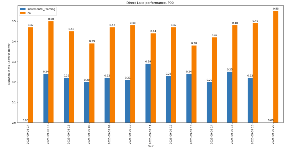
P90
P90 (90th percentile latency):
Less dramatic but still strong.
Improved from 500 ms → 200 ms.
Faster queries also reduce capacity unit usage.
Geomean
just for fun and to show how fast Vertipaq is, let’s see the geomean, alright went from 11 ms to 8 ms, general purpose OLAP engines are cool, but specialized Engines are just at another level !!!
This does not solve Bad Table layout problem
This feature improves support for Delta tables with frequent appends and deletes. However, performance still degrades if you have too many small Parquet row groups.
VertiPaq does not rewrite data layouts—it reads data as-is. To maintain good performance:
Compact your tables regularly.
In my case, I backfill data nightly. The small Parquets added during the day don’t cause major issues, but I still compact every 100 files as a precaution.