I was giving a presentation about Microsoft Fabric Python notebooks and someone asked if they scale. The short answer is yes. You can download the notebook and try it for yourself. For the long answer, keep reading.
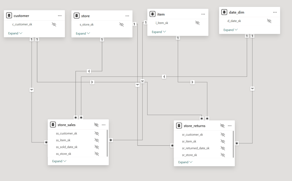
The dataset I used contains the last seven years of Australian electricity market data. Although it’s public, the government agency only keeps archives for two months. I had saved the data during a previous job and kept it around as a hobby. It’s a great real-world workload with realistic data distribution. The CSV files are messy. Technically, they’re more like reports, with different sections stacked on top of each other and varying numbers of columns. That’s often what you encounter in real projects, not the neat, well-structured datasets you see in demos.
For example, being able to read a CSV file with a variable number of columns is a critical feature. Yet this rarely gets mentioned in synthetic benchmarks.
To create a clean environment for testing, I copied the data from one Lakehouse in onelake to a brand-new workspace. I could have used a shortcut, but I wanted to start from scratch. The binary copy took just 2 minutes, with no transformations, which gives a throughput of 1.4 GB per second. That’s pretty good for a 150 GB uncompressed dataset.

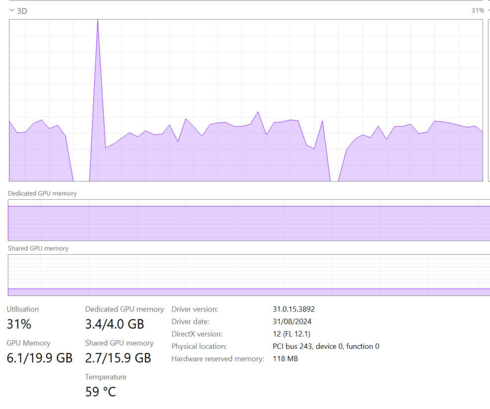
The default configuration for Fabric Python notebooks includes 2 cores and 16 GB of RAM. That’s roughly the same size as Google Colab. But you can easily increase the number of cores to 4, 8, 16, 32, or even 64. At 64 cores, you get nearly half a terabyte of RAM. That’s a serious machine.
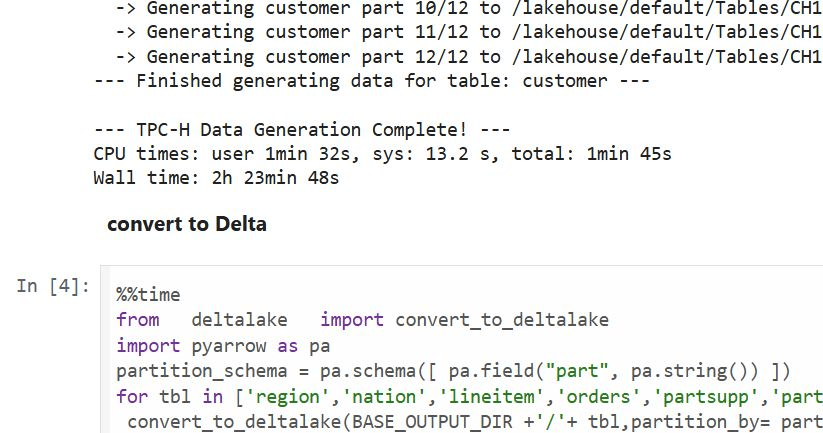
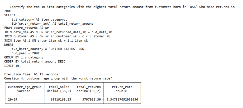
The job itself is simple. Ingest and process the data using several Python engines, then save the result as a Delta table. The raw data has around one billion records, and you end up extracting 311 million. If your engine cannot push down filters to the CSV level, you’re going to have a hard time. The trick here is not to be fast, but to avoid doing unnecessary work.
I used the following engines: DuckDB, Daft, Polars, CHDB (basically ClickHouse for Python), DataFusion, PyArrow, and Pandas. Technically, Pandas is not ideal here because you can’t pass a list of files without using a loop. But I had used it for nearly seven years, so I kept it for sentimental reasons.
I’m fairly confident using all of these engines except PyArrow and DataFusion. Their syntax is very intimidating, and I probably missed some configuration settings. I couldn’t get them to use more than a single thread, so CPU utilization stayed very low.
Results

- Polars support streaming writes, but doesn’t allow exporting a record batch. This means the Delta writer has to load all data into memory. It works fine with 32 cores and 256 GB of RAM, but you’ll run into out-of-memory issues with 16 cores and below.
- Chdb 3.5 added a user friendly way to export arrow record batch, it is the first release so still some bugs, for example got an error with 2 cores, I am sure it will get fixed soon
- Daft is the only engine that supports native writing to Delta. It uses the Deltalake package only to commit the transaction log. The actual Parquet write is handled by the engine itself.
- DuckDB preserves the sort order of the input files. it is trick to appeal to Pandas users who care about index ordering. For best performance though, you should turn this off. (Honestly, I think it should be off by default)
- DuckDB exports Arrow tables by default. You need to explicitly use
record_batch(). I’ve lost count of how many out-of-memory issues I’ve solved just by changing the export format. - Overall, DuckDB delivered the best performance, especially considering it’s not even writing Parquet files directly. It simply streams Arrow data to the writer.
When I first ran the test with DuckDB and saw it finish in under 4 minutes, I thought I made a mistake. It wasn’t until CHDB finished in under 5 minutes that I realized these engines are seriously impressive.
We’re talking about 625 MB per second for processing and ingestion on a single node.
Another key observation: using DuckDB and Daft, even with just 16 GB of RAM, the data was processed correctly. It took about an hour, but it worked without errors, that’s 10 X the size of the RAM
To verify correctness, I simply checked the total sum of a column and the number of records. Everything checked out.

Choosing the Right Size

Now that I know these notebooks work, choosing the right size becomes more nuanced. Surprisingly, the cheapest configuration in term of capacity usage was the 2 cores 🙂
In practice though, using more compute makes sense. A single node has no concept of fault tolerance. If something goes wrong, you need to restart the entire job. Personally, I’m not a fan of long-running jobs. Too many things can go wrong. I used 2 cores just to make a point. That said, using 64 cores doesn’t make much sense either. You’re doubling your compute cost to save 30 seconds.
One more thing: while Daft scales down very well, it doesn’t seem to scale up as efficiently as I had hoped. Ideally, you want a flat performance curve. The total amount of work is fixed, so adding more cores should just reduce execution time. I know the reality is more complex. It’s not easy to keep all processors busy at higher scales.
What This Means
As you may have guessed, I’m a big fan of single-node setups and DuckDB. But I don’t want just one engine to dominate every benchmark or deliver results that no other engine in its class can match. That’s why I was genuinely excited by Daft’s performance. I’m also looking forward to seeing Polars and CHDB add Arrow streaming support.
To be honest, I look at the world from a storage perspective. More competition between engines is a good thing. All of these tools are open source under the MIT license. Most of them can write to Delta in one form or another. and as a user you can choose any engine you want, I think that’s a fantastic thing to have.
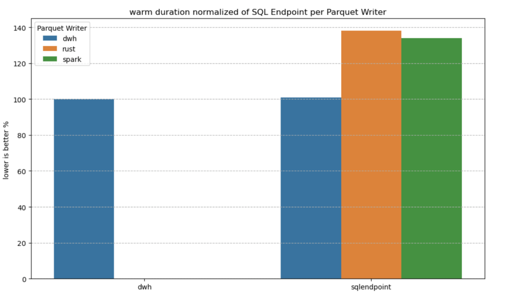
So yes, Python notebooks do scale. The experience is far from being perfect, and there’s still room for improvement. But scalability is not something you should worry about, unless of course you are really doing real big data, then you go distributed 🙂 DWH and Spark are robust options in Fabric.
Edit : tested with chdb 3.5 which has support for arrow streaming