I don’t know much about SQL Server. The closest I ever got to it was having read only access to a database. I remember 10 years ago we had a use case for a database, and IT decided for some reason that we were not allowed to install SQL Server Express. Even though it was free and a Microsoft product. To this day, it is still a mystery to me, anyway, at that time I was introduced to PowerPivot and PowerQuery, and the rest was history.
Although I knew very little about SQL Server, I knew that SQL Server users are in love with the product. I worked with a smart data engineer who had a very clear world view:
I used SQL Server for years. It is rock solid. I am not interested in any new tech.
At the time, I thought he lacked imagination. Now I think I see his point.
When SQL Server was added to Fabric, I was like, oh, that’s interesting. But I don’t really do operational workloads anyway, so I kind of ignored it.
Initially I tried to make it fit my workflow, which is basically developing Python notebooks using DuckDB or Polars (depending on my mood) inside VSCode with GitHub Copilot. and deploy it later into Fabric, of course you can insert a dataframe into SQL Server, but it did not really click for me at first. To be clear, I am not saying it is not possible. It just did not feel natural in my workflow( messing with pyodbc is not fun).
btw the SQL extension inside VSCode is awesome
A week ago I was browsing the DuckDB community extensions and I came across the mssql extension. And boy !!! that was an emotional rollercoaster (The last time I had this experience was when I first used tabular editor a very long time ago).
You just attach a SQL Server database using either username and password or just a token. That’s it. The rest is managed by the extension, suddenly everything make sense to me!!!
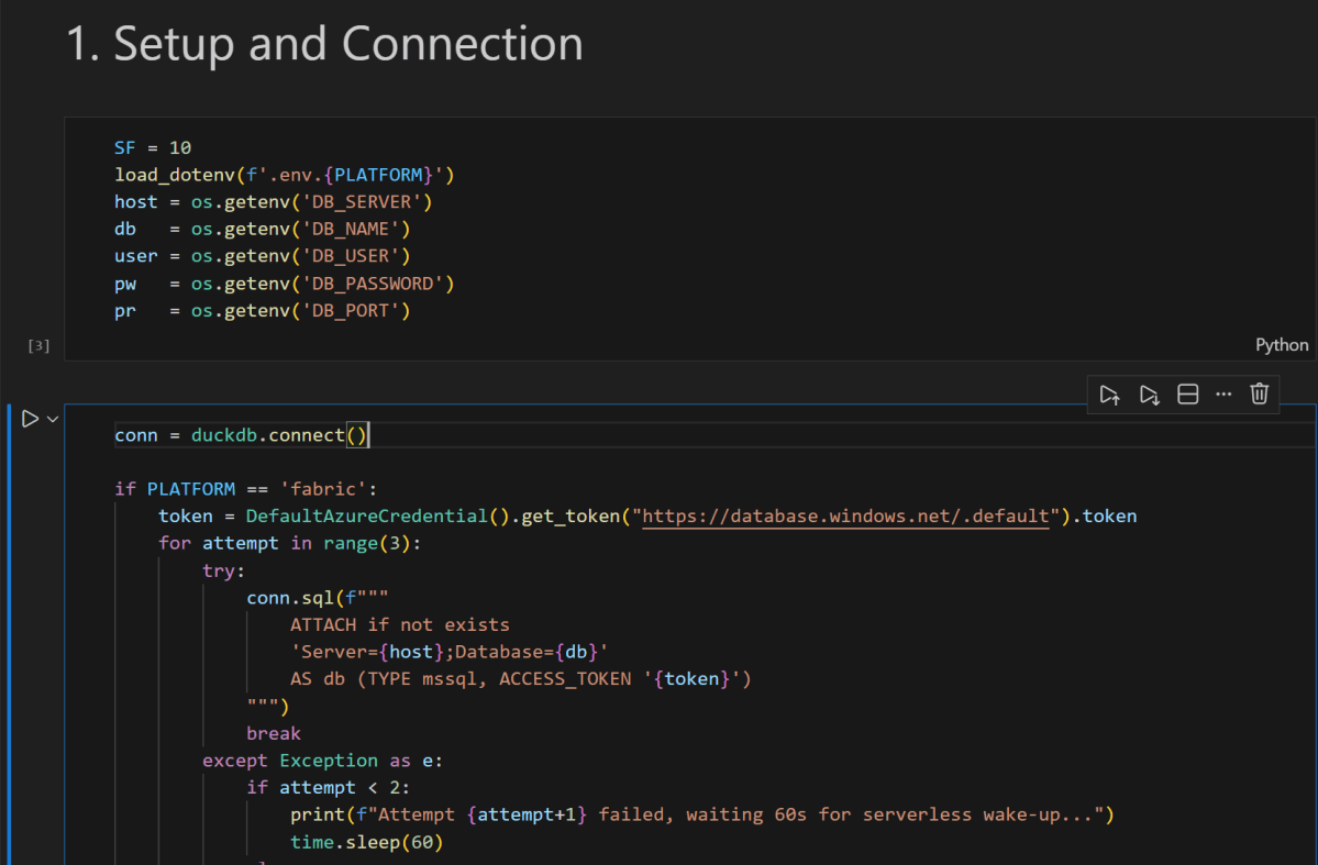
conn = duckdb.connect()

if PLATFORM == 'fabric':
    token = DefaultAzureCredential().get_token("https://database.windows.net/.default").token
# notebookutils.credentials.getToken("sql") inside Fabric notebook
    for attempt in range(3):
        try:
            conn.sql(f"""
                ATTACH IF NOT EXISTS
                'Server={host};Database={db}'
                AS db (TYPE mssql, ACCESS_TOKEN '{token}')
            """)
            break
        except Exception as e:
            if attempt < 2:
                print(f"Attempt {attempt+1} failed, waiting 60s for serverless wake-up...")
                time.sleep(60)
            else:
                raise e
else:
    conn.sql(f"""
        ATTACH OR REPLACE
        'Server={host},{pr};Database={db};User Id={user};Password={pw};Encrypt=yes'
        AS db (TYPE mssql)
    """)

conn.sql("SET mssql_query_timeout = 6000; SET mssql_ctas_drop_on_failure = true;")
print(f"Connected to SQL Server via {PLATFORM}")
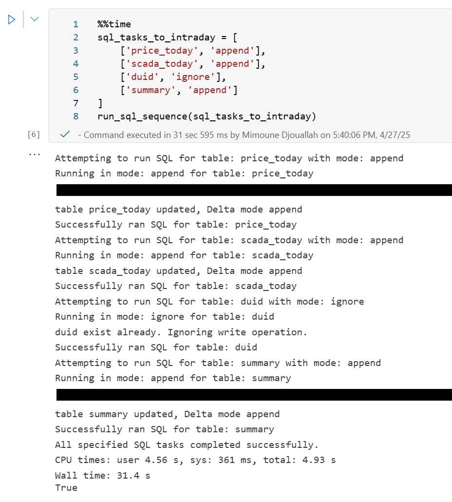
again, I know there other ways to load data which are more efficiently, but if I have a small csv that I processed using python, nothing compare to the simplicity of a dataframe, in that week; here are some things I learned, I know it is obvious for someone who used it !!! but for me, it is like I was living under a rock all these years 🙂
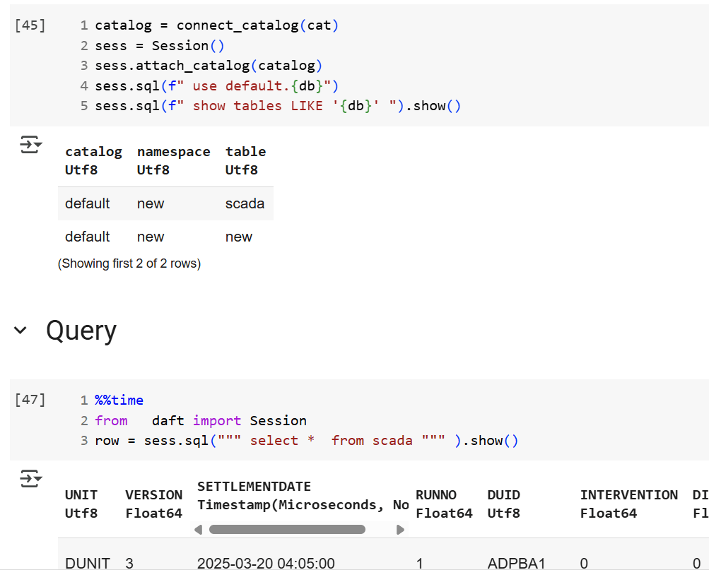
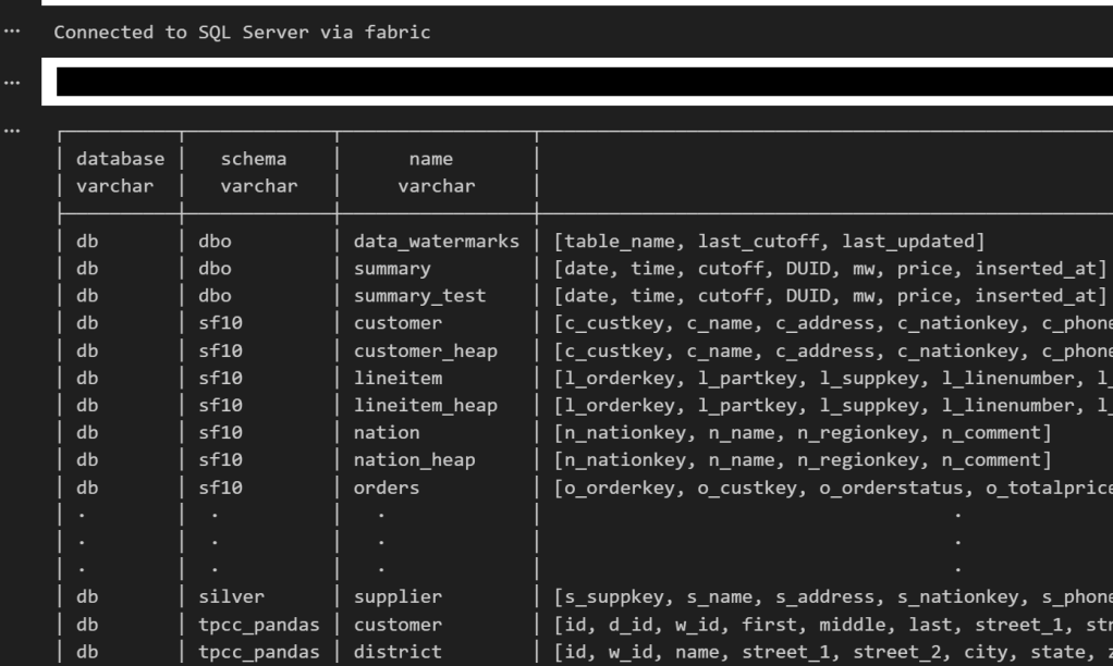
if you run show all tables in duckdb, you get something like this
TDS and bulk insertion
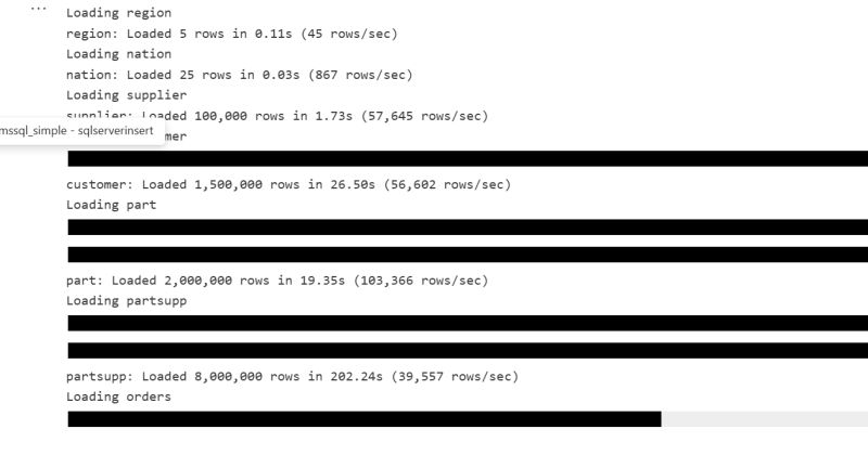
You don’t need ODBC. You can talk to SQL Server directly using TDS, which is the native protocol it understands. There is also something called BCP, which basically lets you batch load data efficiently instead of pushing rows one by one. Under the hood it streams the data in chunks, and the performance is actually quite decent. It is not some hacky workaround. It feels like you are speaking SQL Server’s own language, and that changes the whole experience.
SQL Server is not only for OLTP
Turns out people use SQL Server for analytics too, with columnar table format.
CREATE CLUSTERED COLUMNSTORE INDEX cci_{table}
ON {schema}.{table}
ORDER ({order_col});
I tested a typical analytical benchmark and more or less it performs like a modern single node data warehouse.
Accelerating Analytics for row store
Basically, there is a batch mode where the engine processes row-based tables in batches instead of strictly row by row. The engine can apply vectorized operations, better CPU cache usage, and smarter memory management even on traditional rowstore tables. It is something DuckDB added with great fanfare to accelerate PostgreSQL heap tables. I was a bit surprised that SQL Server already had it for years.
RLS/CLS for untrusted Engine
If you have a CLS or RLS Lakehouse table and you want to query it from an untrusted engine, let’s say DuckDB running on your laptop, today, you can’t for a good reason as the direct storage access is blocked, this extension solves it, as you query the SQL Endpoint itself.
Most of fancy things were already invented
Basically, many of the things’ people think are next generation technologies were already implemented decades ago. SQL control flow, temp tables, complex transactions, fine grained security, workload isolation, it was all already there.
I think the real takeaway for me; user experience is as important – if not more- than the SQL Engine itself, and when a group of very smart people like something then there is probably a very good reason for it.