There are moments in life when you know things will never be the same. I remember distinctly when Gary showed me PowerPivot 10 years ago, and I knew that working with data would become as easy as playing with Excel. Another such moment was two days ago when I connected Claude Desktop to a database and asked, “What do you think?”
It was a strange experience. It wasn’t your typical “chat with your data and give me a nice chart” interaction. It was more like talking to a human and asking them to create a report. The LLM started by listing all the tables, examining the data, and making sense of what the dataset was about. Somehow, it figured out that the power generation figures were in MW and that to convert them to MWh, you need to divide by 12.
There’s a simple reason why this approach is so powerful compared to a typical chat with your data workflow: the LLM has read access to the data. It’s still secure and can only read what you’re authorized to access. As far as I know, these LLMs don’t auto-learn and don’t use the data for training, at least when you use an enterprise API.
Another interesting observation: as a non-programmer, I watched AI’s progress in coding with great excitement and never felt much sympathy for human coders. I thought they were exaggerating the threat. Somehow, my reaction changed when I noticed that AI will get very good at analytics too.
Note: I’ll refer to LLMs as AI for simplicity. Kurt has an excellent blog post worth reading, and thanks to Pawel for telling me about this whole MCP thing.
Typical “Chat with Your Data” Workflow

The important thing here is that AI doesn’t have access to your data at all. You collect the maximum knowledge about your data and send your questions with that knowledge. You get back SQL or DAX statements that you send to your server to get answers. if the question is not clear enough then they will ask for clarification, for example, what is the biggest country in the world, AI will reply, is it per size, by GDP etc, It’s much more complex in real life, but that’s the core idea.
Basically, we spend a lot of effort making sure AI can’t see your data. Sometimes, as a user, you wonder why this AI can’t answer some very obvious questions. Just imagine: as a data analyst, if someone asked you to give them a report without even seeing any numbers!
Using MCP

In this setup, the AI is unleashed. It can read the data directly (again, using only what you’re allowed to access and ideally read only), basically AI acts like an agent and has more autonomy, it is not limited only to your metadata.
Example Using Data from OneLake
I have this data in OneLake, and it’s cleansed data:

Because we don’t have an MCP server yet for Fabric DWH, I used the DuckDB MCP server to read the data from OneLake. For convenience, instead of using direct query, I imported the data into a local DuckDB file:
import duckdb

con = duckdb.connect()
con.sql("ATTACH 'aemo_delta.duckdb' AS db; USE db")

for tbl in ['duid', 'summary', 'calendar', 'mstdatetime']:
    con.sql(f"""
        CREATE OR REPLACE TABLE {tbl} AS
        FROM delta_scan('abfss://serving@onelake.dfs.fabric.microsoft.com/datamart.Lakehouse/Tables/aemo/{tbl}')
    """)

con.close()
You need to install MCP and configure the connection with Claude Desktop. To be clear, it should work with any MCP client, but so far, that’s the best I could find. Who knows, maybe one day Power BI Desktop will act as an MCP client (I literally made up this idea; this is not a hint or anything).
Then you add this config to Claude Desktop:
{
  "mcpServers": {
    "mcp-server-motherduck": {
      "command": "uvx",
      "args": [
        "mcp-server-motherduck",
        "--db-path",
        "/tmp/llm/aemo_delta.duckdb"
      ]
    }
  }
}
For me, it feels like ODBC for AI. The protocol is getting adopted by everyone.
The Experience
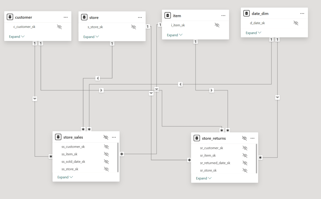
Since the data is public, I shared the whole chat. What I really like is how AI approaches the problem, first by looking at the tables. This is very human-like behavior.

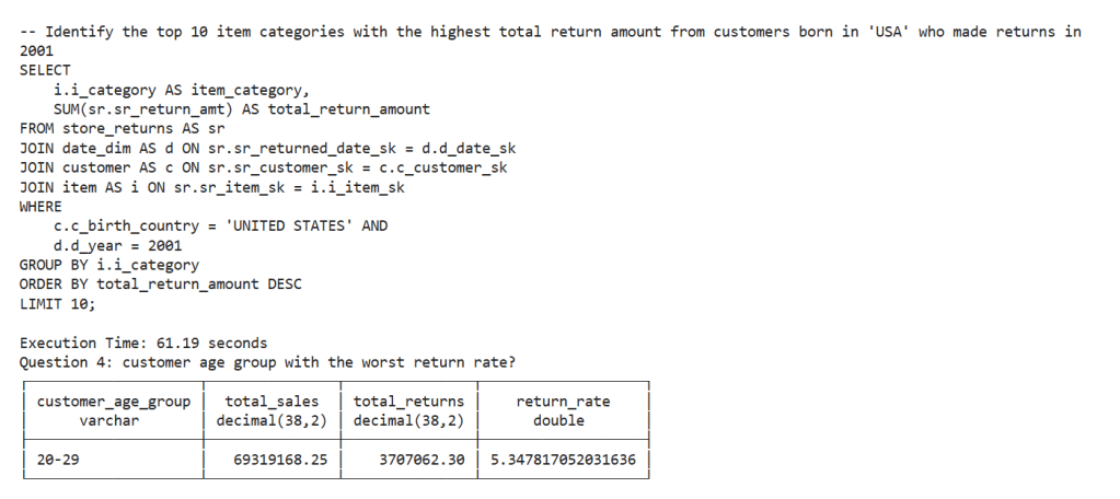
If you read the chat, you’ll see it’s not perfect. It casually skipped hydro from the renewable conversation and didn’t calculate MWh correctly, although it did yesterday.

Some Observations
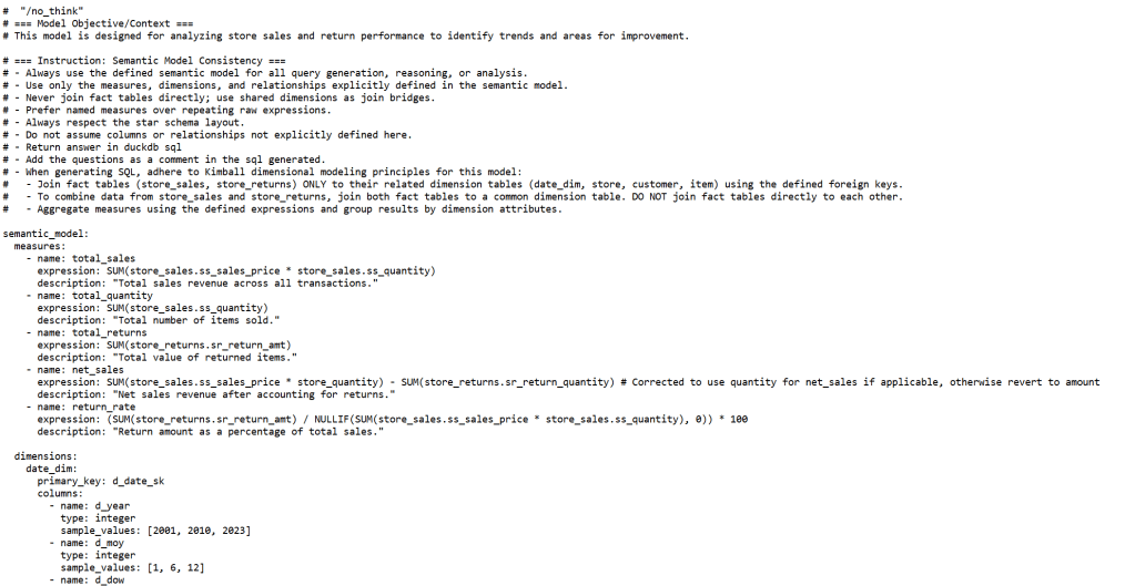
- Even for a simple use case, you still need a semantic model. If I had a measure MWh = MW/12, the AI would always use it, at least in theory. For a complex model, it’s even more critical, Having said that, AI can do modeling just fine 🙂 do we need human for that ?
- surprisingly in that simple workflow, i can replace every compute , what’s really critical is storage !!!
- All my data is publicly available, so I wasn’t worried about security. For any enterprise work, you can’t really use something like Claude Desktop, but rather solutions like Azure AI Foundry.
- For now, most models don’t acquire new knowledge during serving, but who knows what will happen in the next 10 years? You can imagine an AI that learns just from interaction with users and data, which opens all kinds of new questions. Do you need specific models for every tenant, for every user ? We’re not there yet, it is something we will have to deal with it.
- Never give MCP write access to anything