If you’ve ever worked with Delta tables, for example using delta_rs, you know that writing to one is as simple as passing the URL and credentials. It doesn’t matter whether the URL points to OneLake, S3, Google Cloud, or any other major object store — the process works seamlessly. The same applies whether you’re writing data using Spark or even working with Iceberg tables.
However, things get complicated when you try to list a bucket or copy a file. That’s when the chaos sets in. There is no standard method for these tasks, and every vendor has its own library. For instance, if you have a piece of code that works with S3, and you want to replicate it in Azure, you’ll need to rewrite it from scratch.
This is where OpenDalcomes in. OpenDal is an open-source library written in Rust (with Python bindings) that aims to simplify this problem. It provides a unified library to abstract all object store primitives, offering the same API for file management across multiple platforms (or “unstructured data” if you want to sound smart). While the library has broader capabilities, I’ll focus on this particular aspect for now.
I tested OpenDal with Azure ADLS Gen2, OneLake, and Cloudflare R2. To do so, I created a small Python notebook (with the help of ChatGPT) that syncs any local folder to remote storage. It works both ways: if you add a file to the remote storage, it gets replicated locally as well.
Currently, there’s a limitation: OpenDal doesn’t work with OneLake yet, as it doesn’t support OAuth tokens, and SAS tokens have a limited functionality ( it is by design, you can’t list a container for example from OneLake)
you need just to define your object store and the rest is the same, list, create folder, copy, write etc all the same !!! this is really a very good job
While experimenting with different access modes in Power BI, I thought it is maybe worth sharing as a short blog to show why the Lakehouse architecture offers versatile options for Power BI developers. Even when they use Only Import Mode.
And Instead of sharing a conceptual piece, perhaps focus on presenting some dollar figures 🙂
Scenario: A Small Consultancy
According to local regulations, a small enterprise is defined as having fewer than 15 employees. Let’s consider this setup:
Data Storage: The data resides in Microsoft OneLake, utilizing an F2 SKU.
Number of Users: 15 employees.
Data Size: Approximately 94 million rows.
Pricing Model: For simplicity, assume the F2 SKU uses a reserved pricing model.
Monthly Costs:
Power BI Licensing: 15 users × 15 AUD = 225 AUD.
F2 SKU Reserved Pricing: 293 AUD.
Total Cost: 518 AUD per month.
ETL Workload
Currently, the ETL workload consumes approximately 50% of the available capacity.
For comparison, I ran the same workload on another Lakehouse vendor. To minimize costs, the schedule was adjusted to operate only from 8 AM to 6 PM. Despite this adjustment, the cost amounted to:
Daily Cost: 40 AUD.
Monthly Cost: 1,200 AUD.
In contrast, the F2 SKU’s reserved price of 293 AUD per month is significantly more economical. Even the pay-as-you-go model, which costs 500 AUD per month, remains competitive.
Key Insight:
While serverless billing is attractive, what matter is how much you end up paying per month.
For smaller workloads (less than 100 GB of data), data transformation becomes commoditized, and charging a premium for it is increasingly challenging.
Analytics in Power BI
I prefer to separate Power BI reports from the workspace used for data transformation. End users care primarily about clean, well-structured tables—not the underlying complexities.
With OneLake, there are multiple ways to access the stored data:
Import Mode: Directly import data from OneLake.
DirectQuery: Use the Fabric SQL Endpoint for querying.
Direct Lake Model: Access data with minimal latency.
Composite Models: All the above ( this is me trying to be funny)
All the Semantic Models and reports are hosted in the Pro license workspace, Notice that an import model works even when the capacity is suspended ( if you are using pay as you go pricing)
The Trade-Off Triangle
In analytical databases, including Power BI, there is always a trade-off between cost, freshness, and query latency. Here’s a breakdown:
Import Mode: Ideal if eight refreshes per day suffice and the model size is small. Reports won’t consume Fabric capacity (Onelake Transactions cost are insignificant for small data import)
Direct Lake Model: Provides excellent freshness and latency but will probably impacts F2 capacity, in other words, it will cost more.
DirectQuery: Balances freshness and latency (seconds rather than milliseconds) while consuming less capacity. This approach is particularly efficient as Fabric treats those Queries as background operations, with low consumption rates in many cases. Looking forward to the release of Fabric DWH result cache.
Key Takeaways
Cost-Effectiveness: Reserved pricing for smaller Fabric F SKUs combined with Power BI Pro license offers a compelling value proposition for small enterprises.
Versatility: OneLake provides flexible options for ETL workflows, even when using import mode exclusively.
The Lakehouse architecture and Power BI’s diverse access modes make it possible to efficiently handle analytics, even for smaller enterprises with limited budgets.
As the year comes to a close, I decided to explore a fun yet somewhat impractical challenge: Can DuckDB run the TPC-DS benchmark using just 2 cores and 16 GB of RAM? The answer is yes, but with a caveat—it’s slow. Despite the limitations, it works!
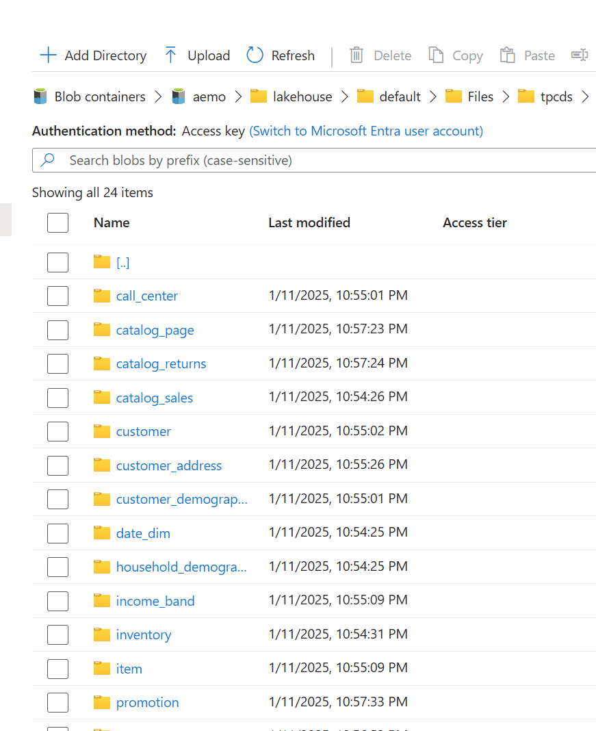
Notice; I am using lakehouse mounted storage, for a background on the different access mode, you can read the previous blog
Data Generation Challenges
Initially, I encountered an out-of-memory error while generating the dataset. Upgrading to the development release of DuckDB resolved this issue. However, the development release currently lacks support for reading Delta tables, as Delta functionality is provided as an extension available only in the stable release.
Here are some workarounds:
Increase the available RAM.
Use the development release to generate the data, then switch back to version 1.1.3 for querying.
Wait for the upcoming version 1.2, which should resolve this limitation.
The data is stored as Delta tables in OneLake, it was exported as a parquet files by duckdb and converted to delta table using delta_rs (the conversion was very quick as it is a metadata only operation)
Query Performance
Running all 99 TPC-DS queries worked without errors, albeit very slowly( again using only 2 cores ).
I also experimented with different configurations:
4, 8, and 16 cores: Predictably, performance improved as more cores were utilized.
For comparison, I ran the same test on my laptop, which has 8 cores and reads my from local SSD storage, The Data was generated using the same notebook.
Results
Python notebook compute consumption is straightforward, 2 cores = 1 CUs, the cheapest option is the one that consume less capacity units, assuming speed of execution is not a priority.
Cheapest configuration: 8 cores offered a good balance between cost and performance.
Fastest configuration: 16 cores delivered the best performance.
Interestingly, the performance of a Fabric notebook with 8 cores reading from OneLake was comparable to my laptop with 8 cores and an SSD. This suggests that OneLake’s throughput is competitive with local SSDs.
Honestly, It’s About the Experience
At the end of the day, it’s not just about the numbers. There’s a certain joy in using a Python notebook—it just feels right. DuckDB paired with Python creates an intuitive, seamless experience that makes analytical work enjoyable. It’s simply a very good product.
Conclusion
While this experiment may not have practical applications, it highlights DuckDB’s robustness and adaptability. Running TPC-DS with such limited resources showcases its potential for lightweight analytical workloads.
This is not an official benchmark—just an exercise to experiment with the new Fabric Python notebook.
You can download the notebook and the results here
There is a growing belief that most structured data will eventually be stored in an open table format within object stores, with users leveraging various engines to query that data. The idea of data being tied to a specific data warehouse (DWH) may soon seem absurd, as everything becomes more open and interoperable.
While I can’t predict the future, 2024 will likely be remembered as the year when the lakehouse concept decoupled from Spark. It has become increasingly common for “traditional” DWHs or any Database for that matter to support open table formats out of the box. Fabric DWH, for instance, uses a native storage layer based on Parquet and publishes Delta tables for consumption by other engines. Snowflake now supports Iceberg, and BigQuery is slowly adding support as well.
I’m not particularly worried about those DWH engines—they have thousands of engineers and ample resources, they will be doing just fine.
My interest lies more in the state of open source Python engines, such as Polars and DataFusion, and how they behave with a limited resource environment.
Benchmarking Bias
Any test inherently involves bias, whether conscious or unconscious. For interactive queries, SQL is the right choice for me. I’m aware of the various DataFrame APIs, but I’m not inclined to learn a new API solely for testing. For OLAP-type queries, TPC-DS and TPC-H are the two main benchmarks. This time, I chose TPC-DS for reasons explained later.
Benchmark Setup
All data is stored in OneLake’s Melbourne region, approximately 1,400 km away from my location, the code will check if the data exists otherwise it will be generated, the whole thing is fully reproducible.
I ran each query only once, ensuring that the DuckDB cache, which is temporary, was cleared between sessions. This ensures a fair comparison.
I explicitly used the smallest available hardware since larger setups could mask bottlenecks. Additionally, I have a specific interest in the Fabric F2 SKU.
While any Python library can be used, as of this writing, only two libraries—DuckDB and DataFusion—support:
Running the 99 TPC-DS queries (DataFusion supports 95, which is sufficient for me).
Native Delta reads for abfss or at least local paths.
Python APIs, as they are required to run queries in a notebook.
Other libraries like ClickHouse, Databend, Daft, and Polars lack either mature Delta support or compatibility with complex SQL benchmarks like TPC-DS.
Why TPC-DS ?
TPC-DS presents a significantly greater challenge than TPC-H, with 99 queries compared to TPC-H’s 22. Its more complex schema, featuring multiple fact and dimension tables, provides a richer and more demanding testing environment.
Why 10GB?
The 10GB dataset reflects the type of data I encountered as a Power BI developer. My focus is more on scaling down than scaling up. For context:
The largest table contains 133 million rows.
The largest table by size is 1.1GB.
Admittedly, TPC-DS 10GB is overkill since my daily workload was around 1GB. However, running it on 2 cores and 16GB of RAM highlights DuckDB’s engineering capabilities.
btw, I did run the same test using 100GB and the python notebook with 16 GB did works just fine, but it took 45 minutes.
OneLake Access Modes
You can query OneLake using either abfss or mounted storage. I prefer the latter, as it simulates a local path and libraries don’t require authentication or knowledge of abfss. Moreover, it caches data on runtime SSDs, which is an order of magnitude faster than reading from remote storage. Transactions are also included in the base capacity unit consumption, eliminating extra OneLake costs.
It’s worth noting that disk storage in Fabric notebook is volatile and only available during the session, while OneLake provides permanent storage.
You can read more about how to laverage DuckDB native storage format as a cache layer here
Onelake Open internet throughput
My internet connection is not too bad but not great either, I managed to get a peak of 113 Mbps, notice here the extra compute of my laptop will not help much as the bottleneck is network access.
Results
The table below summarizes the results across different modes, running both in Fabric notebooks and on my laptop.
DuckDB Disk caching yielded the shortest durations but the worst individual query performance, as copying large tables to disk takes time.
Delta_rs SQL performance was somewhat erratic.
Performance on my laptop was significantly slower, influenced by my internet connection speed.
Mounted storage offered the best overall experience, caching only the Parquet files needed for queries.
And here is the geomean
Key Takeaways
For optimal read performance, use mounted storage.
For write operations, use the abfss path.
Having a data center next to your laptop is probably a very good idea 🙂
Due to network traffic, Querying inside the same region will be faster than Querying from the web (I know, it is a pretty obvious observation)
but is Onelake throughput good ?
I guess that’s the core question, to answer that I changed the Python notebook to use 8 cores, and run the test from my laptop using the same data stored in my SSD Disk, no call to onelake, and the results are just weird
Reading from Onelake using mounted storage in Fabric Notebook is faster than reading the same data from my Laptop !!!!
Looking Ahead to 2025
2024 has been an incredible year for Python engines, evolving from curiosities to tools supported by major vendors. However, as of today, no single Python library supports disk caching for remote storage queries. This remains a gap, and I hope it’s addressed in 2025.
For Polars and Daft, seriously works on better SQL support