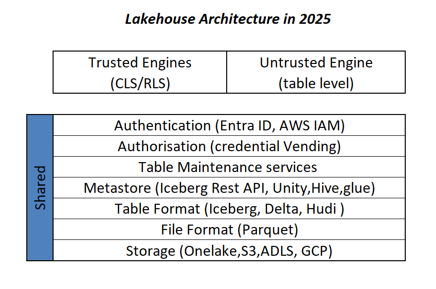
This is more or less the industry consensus on how a Lakehouse architecture should look in 2025.
By now, it’s become clear that Parquet is the de facto standard for storing data, and using an object store to separate storage from compute makes a lot of sense.
Another interesting development is how vendors want to package this offering. Storage vendors saw an opportunity to do more—after all, there’s no law that says the metastore belongs to the data warehouse! So you get things like S3 Table and Cloudflare R2, which I think is a good thing, especially if you’re a smaller analytics vendor. Life becomes much easier when table maintenance is done upstream, allowing you to focus solely on making the query engine faster.
Encouraging things are also happening in the table format space. I know a bit about Iceberg and Delta, but not much about the others. One very interesting development is Iceberg adopting deletion vectors from Delta in the V3 spec, while Delta will requires a catalog for read and write (at least for catalog managed table). I like to call it the “Icebergification” of Delta.
Another trend is the Delta Java writer making it easier to auto-generate Iceberg metadata. and Xtable is doing the same regardless of the delta writer, At this stage, one could argue: why do we need two table formats that are becoming virtually identical?
Data Analyst—How About Me?
These improvements mostly impact the write path, which is primarily managed by data engineers. But what about data analysts and end users?
if you have Fabric OneLake, you can use Direct Lake in OneLake mode. Marco has a great article about it. It’s a fantastic improvement compared to the initial version of Direct Lake. However, it doesn’t solve the problem if your data is hosted in an S3 table or BigQuery Iceberg table. Yes, you can create a shortcut to OneLake and read it from there, but that still depends on a data engineer setting it up.
Now imagine a world where an Excel, Tableau, or Power BI Desktop user (or any arbitrary client tool) can just point to a Lakehouse using a standard API, discover tables, read data, and build reports. Honestly, this isn’t a big ask , we already have this when connecting to databases using ODBC, and I don’t see any technical reason why we can’t have the same experience with Lakehouses.
We Already Have This API
For me, the most promising development in the Lakehouse ecosystem is the Iceberg Catalog REST API, and I genuinely hope it becomes a standard—just like ODBC is today (and hopefully ADBC in the future, but that’s another topic).
Again, speaking as a data analyst, I want my tools to support the read part of the API—just the ability to list tables and scan a table. That’s all. I have zero interest in how the data is stored or which table format is used. The catalog should be smart enough to generate metadata on the fly.
The Good News
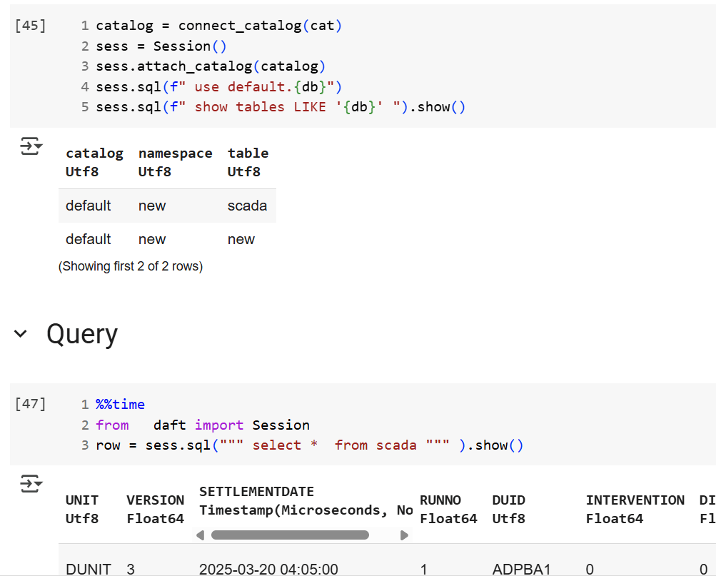
We’re getting there—at least if you’re using a Python notebook. Here’s an example where I use the same Iceberg REST API to query a table from four different Lakehouse implementations using Daft.
def connect_catalog(cat):
  match cat:
    case 'polaris':
      catalog = load_catalog(
              'default',
              uri= polaris_endpoint,
              warehouse='dwh',
              scope = 'PRINCIPAL_ROLE:data_engineer' ,
              credential= polaris_key
            )
    case 's3':
      catalog = load_catalog(
              'default',
              **{
                "type": "rest",
                "warehouse": s3_warehouse ,
                "uri": "https://s3tables.us-east-2.amazonaws.com/iceberg",
                "rest.sigv4-enabled": "true",
                "rest.signing-name": "s3tables",
                "rest.signing-region": "us-east-2"
              }
            )
    case 'uc':
      catalog = load_catalog(
               'default',
              token = token ,
              uri = endpoint,
              warehouse = 'ne'
              )
    case 'r2':
      catalog = RestCatalog(
              name = 'default',
              token = token_r2 ,
              uri = endpoint_r2,
              warehouse = r2_warehouse
              )
  return catalog
Then, I run a standard SQL query using Daft SQL.
Final Thoughts
It took Parquet a decade to become a standard. We may or may not have a single standard table format—and maybe we don’t need one. But if we want this Lakehouse vision to become mainstream, then everyone should support the Iceberg Catalog REST API, at least for read operations.