Using Apache Arrow Dataset to compact old partitions

It is trick I learn today and thought it maybe useful to share, I have a folder of parquet files, partitioned by day using Hive style, the data is ingested every 5 minutes which end up generating 288 small parquet files per day, it is rather nice for a write scenario but reading that data will be slow as it generate a big overhead opening individual files, it is a well documented problem, and more sophisticated table format like Delta Table and Iceberg fix the problem by using compaction, but it does not work with Python. ( Edit by Python, I mean Engine Like Data Fusion, DuckDB , Pandas not Spark which does not make sense for a small Dataset)

In my example I use Only Python and pyarrow dataset which does not support compaction, but maybe there is a solution.

Just for illustration, here is a view of my Bucket in Cloudflare R2 (Pyarrow support S3, GCP and Azure)

Warning : the code will delete existing files, use at your own risk

  • Read the existing partitions except today data, as you may end up having concurrent Write , which will corrupt your table.
  • Filter only the partitions that contains more than 1 file , something like this Using DuckDB
create view base  as select * from  parquet_scan('s3://delta/aemo/scada/data/*/*.parquet' , HIVE_PARTITIONING = 1,filename=1) where Date < '{cut_off}';
create  view  filter as select Date, count(distinct filename) as cnt from  base  group by 1 having cnt>1 
  • Read the data using the previous filter, again, we are not touching today Partition to avoid any conflicts
tb=con.execute('''select SETTLEMENTDATE,DUID,SCADAVALUE,file,cast(base.Date as date) as Date from base inner join filter on base.Date= filter.Date''').arrow()
ds.write_dataset(xx,"delta/aemo/scada/data/", filesystem=s3,format="parquet" , partitioning=['Date'],partitioning_flavor="hive",
     min_rows_per_group=120000,existing_data_behavior="delete_matching")

Again there is no support for transaction, if your code for whatever reason, did not complete, you will end up with unstable table

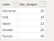
  • And here is the results, all old partitions have only 1 file

You need to run the Job only once a day, hopefully next year sometimes, either Apache Iceberg or Delta Table will provide compaction for the Python client, in the meantime maybe this approach is good enough :), you can see the full code here

Another approach is copy on write, basically every time you ingest a new data, you need to copy the existing data append it to the new data and overwrite existing files, but it maybe an expensive operation, specially if your job runs more frequently.

PowerBI Query plan when using Top N filter

The October release of PowerBI Desktop introduced a very interesting feature, Top N filtered is pushed down for Direct Query Sources, I thought I may give it a try and blog about it, for some reason it did not work, which is great for the purpose of this blog as if you came from a SQL Background you will be surprised how PowerBI DAX Engine Works.

let’s try with one table in BigQuery as an example, and ask this Question, what’s the top 5 Substation by Electricity produced, in PowerBI, it is a trivial exercise, just use the Top N filter

First Observation, 3.7 Second seems rather Slow, BigQuery or any Columnar Database should return the results way faster, specially that we are grouping by low cardinality columns ( around 250 distinct values)

Let’s try SQL Query in BigQuery Console

And let’s check the duration, 351 ms, the table has 91 Million records, that’s not bad at all, but we need to account for the data transfer latency to my laptop, still that does not explain the difference in duration !!!

DAX Engine Query Plan

let’s have a look at the Query Plan generated by DAX Engine using the excellent free tool, DAX Studio

That’s very strange, 2 SQL Query and 1 Second spent by the Formula Engine, and the two SQL Queries are not even in parallel

Looking at the SQL Queries, I think this is the logic of the Query Plan

  • Send a SQL Query to get the list of all the substation and the sum of of MWH.
  • Order the result using the Formula Engine and select 5 substation.
  • Send another SQL Query with a filter of those 5 substation

Probably you are wondering why this convoluted Query Plan, Surely DAX Engine can just send 1 SQL Query to get the results, why the two trips to the source system, which make the whole experience slow.

Vertipaq Don’t support Sort Operator

Vertipaq which is the internal storage engine of PowerBI does not support the sort operator, hence the previous Query do make sense if your Storage engine don’t support sort.

But My Source do support Sorting ?

That’s the new feature, DAX Engine will generate a different plan when the source system do support sorting.

Great, again , Why Vertipaq don’t support sort Operator ?

No idea, probably only a couple of engineers from Microsoft Know the answer.

Edit : 23 October 2022

Jeffrey Wang ( One of the Original Authors of DAX Engine) was very kind and provided this explanation why the optimization did not kick in for BigQuery

Multi fact support in DAX and Malloy

This is a quick blog showing how the two languages behave when dealing with multiple fact tables.

let’s start with a simple Model, Two Tables Budget and Actual storing items sold by country and color

Budget

Actual

For example we want to ask, how many items were sold by continent, we don’t have this information, we need a dimension table that map state to continent.

DAX

And the Data Model will look like this.

To get the results, we write this DAX Query in DAX Studio ( Btw, the new version 3 is very slick !!!)

DAX will generate two SQL Query to get the results from the two tables and merge the results, using the internal “Formula” Engine

Malloy

in Malloy we do the same by writing code, you can download the Data Model here

In DAX we use summarize columns to aggregate measures from different tables, as far as I can tell, Malloy don’t support this model yet, The tables Budget and Actual are independent, basically you need to manually join the two Queries generated from the two tables.

Query: Budget_by_state is Budget -> {
  aggregate:_Budget
  group_by : dim_state.state
}

Query: Actual_by_state is Actual ->{
  aggregate:Quantity
  group_by : dim_state.state
}
query: merge_results is from_sql(state_source_) {
   join_one: q2 is from(->Budget_by_state ) with state
   join_one: q3 is from(->Actual_by_state) with state
} ->{
  
  group_by : continent
  aggregate: QTY_Budget is sum(q2._Budget),QTY_Sold is sum(q3.Quantity)
}

And we get the same results, Malloy always generate one SQL Query, as there is no way to merge the results internally, as a matter of fact the only “calculation” engine is the SQL Database, which is in this particular case DuckDB.

Obviously you can always create new source by using state as a base table, but I don’t think it is a sustainable solution, as the whole point is to have One model that answers a lot of different Questions.

Take Away

Native support to multiple tables is obviously not unique to DAX, thoughtspot TML support it out of the Box, I hope Malloy developers consider this common scenario for future development.

Running a Serverless DuckDB on Google Cloud

TL;DR : it easy to setup and works relatively well, but there is a catch, watch out for Cloud Storage throughput. I shared a notebook here

in previous blog, I showed a POC how to run Queries from a Colab notebook against a delta lake table, but what if you want to run the same Query from other tools, or if you want to run a Query in a different region and avoid egress fees, turn out it is extremely easy to setup.

And here is an Overall View of the architecture. the most important decision is to make sure Cloud Storage and Cloud function are in the same region, in my case “us-central1”, you can call the function from anywhere.

Google Cloud Functions

As I said before the code is very simple, I spent some time googling to convert the results from a byte to json to dataframe, I think beside BigQuery, Google Cloud function is the easiest service to setup, just write your code and Google Cloud handle the rest , just for fun, I used a machine with 8 CPU and 32 GB of RAM.

import pyarrow.dataset as ds
import duckdb
import json
lineitem = ds.dataset("gs://xxxxx/lineitem",format="parquet", partitioning="hive")
con = duckdb.connect()
def Query(request):
    SQL = request.get_json().get('name')
    df = con.execute(SQL).df()
    return json.dumps(df.to_json(orient="records")), 200, {'Content-Type': 'application/json'}

How to Call web API

a lot of tool can send a web api call as long as it has the correct authentication, I started with a python script for a simple reason as it was the easiest to get the code from the internet.

Here is the interesting part, you write any arbitrary SQL code, Then you send an API call, in return you get a json with the results, a user don’t need to know anything about the cloud function, all he needs is the web address and write a correct SQL Query.

Performance considerations

This is where it get very interesting, I have no clue where is the bottleneck, but we can ask some Questions

Cold Start

  • The First example was 334 ms, that’s impressive, but I was cheating, I showed the best case scenario, Google Cloud function or more precisely Cloud Run was already running so no cold start and DuckDB was running a local Query which did not require a call to Cloud storage
  • Currently Cold Start for Cloud run Gen2 is around 10 second, notice it is still in preview.

Transfer from Google Cloud Storage

let’s try this simple Query, we get the result in 29 second

The Same Query using my Laptop, 600 ms, btw table lineitem contains 60 Million rows !!!

I don’t know why the massive difference, I presume network speed is limited, but when I look at the the bucket stats, it is actually very good, nearly 500 MB/S

I am no expert in network, but that number don’t seems right !!, when I check how much Data the cloud function is receiving then the whole discrepancy start making more sense, in average I am getting around 30 MB/s, the maximum was 50 MB/s , I have to say this is really slow !!!

File Pruning

Arrow dataset is smart enough to prune columns that are not used for partitions, in this Query, I made a filter on L_shipdate , notice the parquet file was sorted on that field, and as expected the performance is very good 1.7 second, DuckDB scan only the row groups that contains the date ‘1998-09-02’

Dataset Catalog

I am defining a very rudimentary catalog, the user can just call ” Show Tables”

You can even check the table schema

Cloud Storage throughput is the bottleneck.

having a speed of 30 MB/S make the whole setup just good for POC or doing a Query on a small dataset , I don’t know the reason why such a poor performance from Cloud Run, I suspect Apache arrow implementation is not optimized for GCP although it works very well in a local file system.

Another missing piece is the lack of cache, it would have being good if somehow DuckDB cache the data already Queried, but cache is very hard to implement specially if you want cache invalidation, and you risk reinventing a full Data warehouse. I genuinely hope it is a bug and cloud run can provide a better network performance.